

278
Yoshinari Tanaka
F t+1 = {1/(2N) + [1 − 1/(2N)]F t }(1 − 2µ)(1 − sq)
(Tanaka 1997, 1998).
Equilibrium
Without demographic disturbance and environmental stochasticity, the population
is maintained at a demographic and genetic equilibrium, in which population size,
mean gene frequency, and inbreeding coefficient are constant. These equilibrium
values were used as the initial values of F and q in the simulations. It was assumed
that the population had been at a long-term equilibrium before anthropogenic
factors started to continually degrade populations and disrupt the equilibria.
The long-term effective population size of a stochatically fluctuating population is smaller than the census population size. If there is no autocorrelation in the
fluctuations, the effective population size N e is N − σ
2
N /N, where σ
2
N is the variance
of population size (Crow and Kimura 1970). If the variance is mostly due to
environmental fluctuation in the population growth rate, it is equivalent to σ
2
N =
(σ
2
e K
2 + K)/(2r), where σ
2
e is the environmental variance of the intrinsic rate of
natural increase r (Iwasa 1998). For numerical evaluation of equilibrium values of
inbreeding coefficient and mean gene frequency, the effective population size was
used in place of the population size.
The equilibrium mean gene frequency resulting from the balance between
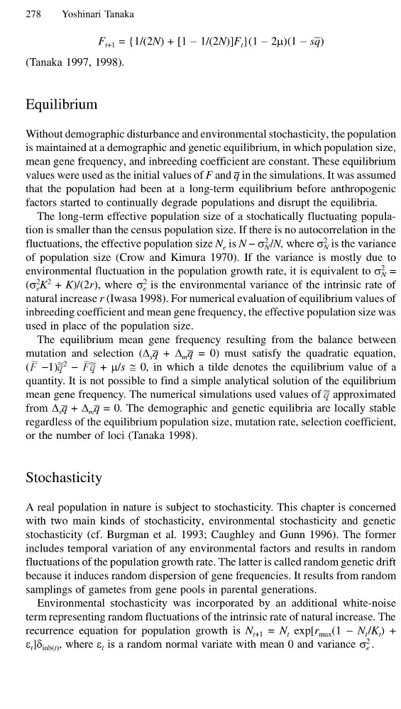
mutation and selection (∆ s q + ∆ m q = 0) must satisfy the quadratic equation,
( −1)
2
−
+ µ/s ≅ 0, in which a tilde denotes the equilibrium value of a
quantity. It is not possible to find a simple analytical solution of the equilibrium
mean gene frequency. The numerical simulations used values of approximated
from ∆ s q + ∆ m q = 0. The demographic and genetic equilibria are locally stable
regardless of the equilibrium population size, mutation rate, selection coefficient,
or the number of loci (Tanaka 1998).
Stochasticity
A real population in nature is subject to stochasticity. This chapter is concerned
with two main kinds of stochasticity, environmental stochasticity and genetic
stochasticity (cf. Burgman et al. 1993; Caughley and Gunn 1996). The former
includes temporal variation of any environmental factors and results in random
fluctuations of the population growth rate. The latter is called random genetic drift
because it induces random dispersion of gene frequencies. It results from random
samplings of gametes from gene pools in parental generations.
Environmental stochasticity was incorporated by an additional white-noise
term representing random fluctuations of the intrinsic rate of natural increase. The
recurrence equation for population growth is N t+1 = N t exp[r max (1 − N t /K t ) +
ε t ]δ inb(t) , where ε t is a random normal variate with mean 0 and variance σ
2
e .
Yoshinari Tanaka
F t+1 = {1/(2N) + [1 − 1/(2N)]F t }(1 − 2µ)(1 − sq)
(Tanaka 1997, 1998).
Equilibrium
Without demographic disturbance and environmental stochasticity, the population
is maintained at a demographic and genetic equilibrium, in which population size,
mean gene frequency, and inbreeding coefficient are constant. These equilibrium
values were used as the initial values of F and q in the simulations. It was assumed
that the population had been at a long-term equilibrium before anthropogenic
factors started to continually degrade populations and disrupt the equilibria.
The long-term effective population size of a stochatically fluctuating population is smaller than the census population size. If there is no autocorrelation in the
fluctuations, the effective population size N e is N − σ
2
N /N, where σ
2
N is the variance
of population size (Crow and Kimura 1970). If the variance is mostly due to
environmental fluctuation in the population growth rate, it is equivalent to σ
2
N =
(σ
2
e K
2 + K)/(2r), where σ
2
e is the environmental variance of the intrinsic rate of
natural increase r (Iwasa 1998). For numerical evaluation of equilibrium values of
inbreeding coefficient and mean gene frequency, the effective population size was
used in place of the population size.
The equilibrium mean gene frequency resulting from the balance between
mutation and selection (∆ s q + ∆ m q = 0) must satisfy the quadratic equation,
( −1)
2
−
+ µ/s ≅ 0, in which a tilde denotes the equilibrium value of a
quantity. It is not possible to find a simple analytical solution of the equilibrium
mean gene frequency. The numerical simulations used values of approximated
from ∆ s q + ∆ m q = 0. The demographic and genetic equilibria are locally stable
regardless of the equilibrium population size, mutation rate, selection coefficient,
or the number of loci (Tanaka 1998).
Stochasticity
A real population in nature is subject to stochasticity. This chapter is concerned
with two main kinds of stochasticity, environmental stochasticity and genetic
stochasticity (cf. Burgman et al. 1993; Caughley and Gunn 1996). The former
includes temporal variation of any environmental factors and results in random
fluctuations of the population growth rate. The latter is called random genetic drift
because it induces random dispersion of gene frequencies. It results from random
samplings of gametes from gene pools in parental generations.
Environmental stochasticity was incorporated by an additional white-noise
term representing random fluctuations of the intrinsic rate of natural increase. The
recurrence equation for population growth is N t+1 = N t exp[r max (1 − N t /K t ) +
ε t ]δ inb(t) , where ε t is a random normal variate with mean 0 and variance σ
2
e .