

132
Danny C. Lee
can be entered at any combination of nodes and the belief vectors of all nodes
updated accordingly via belief propagation. During belief propagation, information is passed along two separate pathways. Thus, a change in belief about a
certain node can originate from a parent node (causal evidence) or a child node
(diagnostic evidence). Causal evidence can be viewed conceptually as prior probabilities in a classical Bayesian application, whereas diagnostic evidence is comparable with sample data. Properly constructed networks recognize where information enters the system and update all other nodes according to the information
received but prevent the updates from changing the belief vector of the originating
node. This prevents circular reasoning (e.g., evidence for smoke leads to increased
belief in the presence of fire, which leads to increased belief in the presence of
smoke, which leads to increased belief in fire, and so on).
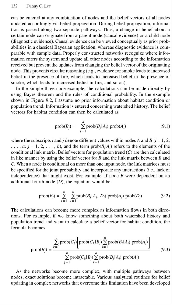
In the simple three-node example, the calculations can be made directly by
using Bayes theorem and the rules of conditional probability. In the example
shown in Figure 9.2, I assume no prior information about habitat condition or
population trend. Information is entered concerning watershed history. The belief
vectors for habitat condition can then be calculated as
prob(B j ) =
a
͚
i =1
prob(B j | A i ) prob(A i )
(9.1)
where the subscripts i and j denote different values within nodes A and B (i = 1, 2,
. . . , a; j = 1, 2, . . . , b), and the term prob(B j |A i ) refers to the elements of the
conditional link matrix. Belief vectors for population trend (C) are then calculated
in like manner by using the belief vector for B and the link matrix between B and
C. When a node is conditional on more than one input node, the link matrices must
be specified for the joint probability and incorporate any interactions (i.e., lack of
independence) that might exist. For example, if node B were dependent on an
additional fourth node (D), the equation would be
prob(B j ) =
a
͚
i =1
d
͚
l =1
prob(B j | A i , D l ) prob(A i ) prob(D l )
(9.2)
The calculations can become more complex as information flows in both directions. For example, if we know something about both watershed history and
population trend and want to calculate a belief vector for habitat condition, the
formula becomes
c
͚
k =1
prob(C k )
΄
prob(C k | B j )
a
͚
i =1
prob(B j | A i ) prob(A i )
΅
prob(B j ) =
(9.3)
b
͚
j =1
prob(C k | B j )
a
͚
i =1
prob(B j | A i ) prob(A i )
As the networks become more complex, with multiple pathways between
nodes, exact solutions become intractable. Various analytical routines for belief
updating in complex networks that overcome this limitation have been developed
Danny C. Lee
can be entered at any combination of nodes and the belief vectors of all nodes
updated accordingly via belief propagation. During belief propagation, information is passed along two separate pathways. Thus, a change in belief about a
certain node can originate from a parent node (causal evidence) or a child node
(diagnostic evidence). Causal evidence can be viewed conceptually as prior probabilities in a classical Bayesian application, whereas diagnostic evidence is comparable with sample data. Properly constructed networks recognize where information enters the system and update all other nodes according to the information
received but prevent the updates from changing the belief vector of the originating
node. This prevents circular reasoning (e.g., evidence for smoke leads to increased
belief in the presence of fire, which leads to increased belief in the presence of
smoke, which leads to increased belief in fire, and so on).
In the simple three-node example, the calculations can be made directly by
using Bayes theorem and the rules of conditional probability. In the example
shown in Figure 9.2, I assume no prior information about habitat condition or
population trend. Information is entered concerning watershed history. The belief
vectors for habitat condition can then be calculated as
prob(B j ) =
a
͚
i =1
prob(B j | A i ) prob(A i )
(9.1)
where the subscripts i and j denote different values within nodes A and B (i = 1, 2,
. . . , a; j = 1, 2, . . . , b), and the term prob(B j |A i ) refers to the elements of the
conditional link matrix. Belief vectors for population trend (C) are then calculated
in like manner by using the belief vector for B and the link matrix between B and
C. When a node is conditional on more than one input node, the link matrices must
be specified for the joint probability and incorporate any interactions (i.e., lack of
independence) that might exist. For example, if node B were dependent on an
additional fourth node (D), the equation would be
prob(B j ) =
a
͚
i =1
d
͚
l =1
prob(B j | A i , D l ) prob(A i ) prob(D l )
(9.2)
The calculations can become more complex as information flows in both directions. For example, if we know something about both watershed history and
population trend and want to calculate a belief vector for habitat condition, the
formula becomes
c
͚
k =1
prob(C k )
΄
prob(C k | B j )
a
͚
i =1
prob(B j | A i ) prob(A i )
΅
prob(B j ) =
(9.3)
b
͚
j =1
prob(C k | B j )
a
͚
i =1
prob(B j | A i ) prob(A i )
As the networks become more complex, with multiple pathways between
nodes, exact solutions become intractable. Various analytical routines for belief
updating in complex networks that overcome this limitation have been developed