

9. Assessing Land-Use Impacts on Bull Trout Using Bayesian Belief Networks
133
by Henrion (1986), Pearl (1988), Lauritzen and Spiegelhalter (1988), and Andersen and associates (1989).
Relatively simple BBNs can be programmed by using spreadsheets or other
software packages that easily manipulate matrices. More complex networks generally are beyond the programming skills or patience of many potential developers. Sophisticated software such as the Hugin system (http://www.hugin.dk),
Netica (http://www.norsys.com), and Analyticia (http://www.lumina.com) provide convenient shells for developing and implementing BBNs with a minimum
of programming. Timothy Haas (University of Wisconsin-Milwaukee, personal
communication) developed a simpler program, BAYES, that is suitable for many
applications. The Hugin system was used for the network presented below; a more
limited spreadsheet version was also developed using Excel.
Bull Trout Network
Three basic steps may be used in assessing land-use impacts on the population
viability of Bull Trout. First, a population viability model is needed that provides a
quantitative assessment of the risk of extinction (or quasi-extinction) given some
combination of population parameters. Second, one must be able to identify
physical changes in habitat conditions that result from land-use activities. The
third and perhaps most problematic step is to link the changes in physical habitat
to the parameters of the viability model.
The overall structure of the Bull Trout BBN is as shown in Figure 9.3. The
intention of introducing it at this point is to help guide the reader through the
following discussion. In essence, I want to use information about the status of a
watershed and the nature of proposed activities to judge the future viability of a
local Bull Trout population. The following sections elaborate on the rationale
behind each node and the linkages among them.
Underlying Viability Model
Some of the best available population data for Bull Trout are time series of counts
of spawning beds (redds). Bull Trout spawn in the fall when stream flows are
generally low. Thus it is relatively easy to observe their spawning redds and obtain
convenient indices of adult population abundance. Rieman and McIntyre’s (1993)
analysis of time series data from northern Idaho and Montana by using the exponential trend model of Dennis and co-workers (1991) suggests high probabilities
of extinction for many of the 19 populations examined. I fit a density-dependent
variant of this model to these same data. The density-dependent model gives a
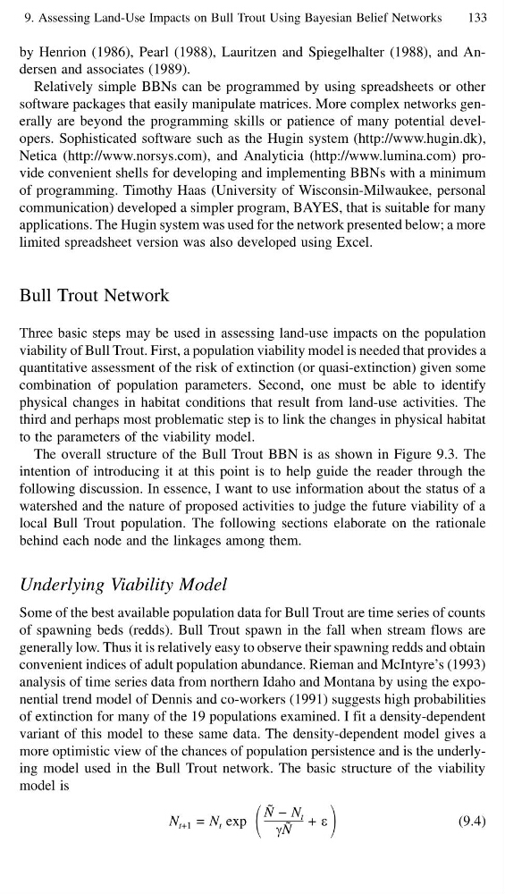
more optimistic view of the chances of population persistence and is the underlying model used in the Bull Trout network. The basic structure of the viability
model is
N t+1 = N t exp
˜
N − N t
γ ˜
N
+ ε
(9.4)
133
by Henrion (1986), Pearl (1988), Lauritzen and Spiegelhalter (1988), and Andersen and associates (1989).
Relatively simple BBNs can be programmed by using spreadsheets or other
software packages that easily manipulate matrices. More complex networks generally are beyond the programming skills or patience of many potential developers. Sophisticated software such as the Hugin system (http://www.hugin.dk),
Netica (http://www.norsys.com), and Analyticia (http://www.lumina.com) provide convenient shells for developing and implementing BBNs with a minimum
of programming. Timothy Haas (University of Wisconsin-Milwaukee, personal
communication) developed a simpler program, BAYES, that is suitable for many
applications. The Hugin system was used for the network presented below; a more
limited spreadsheet version was also developed using Excel.
Bull Trout Network
Three basic steps may be used in assessing land-use impacts on the population
viability of Bull Trout. First, a population viability model is needed that provides a
quantitative assessment of the risk of extinction (or quasi-extinction) given some
combination of population parameters. Second, one must be able to identify
physical changes in habitat conditions that result from land-use activities. The
third and perhaps most problematic step is to link the changes in physical habitat
to the parameters of the viability model.
The overall structure of the Bull Trout BBN is as shown in Figure 9.3. The
intention of introducing it at this point is to help guide the reader through the
following discussion. In essence, I want to use information about the status of a
watershed and the nature of proposed activities to judge the future viability of a
local Bull Trout population. The following sections elaborate on the rationale
behind each node and the linkages among them.
Underlying Viability Model
Some of the best available population data for Bull Trout are time series of counts
of spawning beds (redds). Bull Trout spawn in the fall when stream flows are
generally low. Thus it is relatively easy to observe their spawning redds and obtain
convenient indices of adult population abundance. Rieman and McIntyre’s (1993)
analysis of time series data from northern Idaho and Montana by using the exponential trend model of Dennis and co-workers (1991) suggests high probabilities
of extinction for many of the 19 populations examined. I fit a density-dependent
variant of this model to these same data. The density-dependent model gives a
more optimistic view of the chances of population persistence and is the underlying model used in the Bull Trout network. The basic structure of the viability
model is
N t+1 = N t exp
˜
N − N t
γ ˜
N
+ ε
(9.4)