

7. “Best” Abundance Estimates and Best Management
103
Table 7.2. Base cases for management analysis.
a
Base case
Starting N
R MAX
Survey CV
1
K
0.04
0.2
2
K/3
0.04
0.2
3
K
0.04
0.8
4
K/3
0.04
0.8
5
K
0.12
0.2
6
K/3
0.12
0.2
7
K
0.12
0.8
8
K/3
0.12
0.8
a Cases shown in figures are given in bold type.
equation but constitutes a very different management strategy because it does not
incorporate uncertainty about the level of precision in the abundance estimate.
Analysis of management schemes must consider different types of populations
(different growth rates, initial population status, and different levels of abundance
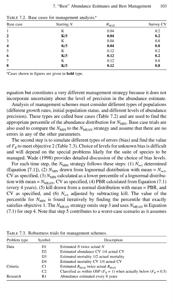
precision). These types are called base cases (Table 7.2) and are used to find the
appropriate percentile of the abundance distribution for N MIN . Base case trials are
also used to compare the N MIN to the N MEAN strategy and assume that there are no
errors in any of the other parameters.
The second step is to simulate different types of errors (bias) and find the value
of F R to meet objective 2 (Table 7.3). Choice of levels for unknown bias is difficult
and will depend on the special problems likely for the suite of species to be
managed. Wade (1998) provides detailed discussion of the choice of bias levels.
For each time step, the N MIN strategy follows these steps: (1) N t+1 determined
(Equation [7.1]), (2) N MIN drawn from lognormal distribution with mean = N t+1 ,
CV as specified, (3) N MIN calculated as a lower percentile of a lognormal distribution with mean = N MEAN , CV as specified, (4) PBR calculated from Equation (7.1)
(every 4 years), (5) kill drawn from a normal distribution with mean = PBR, and
CV as specified, and (6) N t+1 adjusted by subtracting kill. The value of the
percentile for N MIN is found iteratively by finding the percentile that exactly
satisfies objective 1. The N MEAN strategy omits step 3 and uses N MEAN in Equation
(7.1) for step 4. Note that step 5 contributes to a worst-case scenario as it assumes
Table 7.3. Robustness trials for management schemes.
Problem type
Symbol
Description
Data
D1
Estimated N twice actual N
D2
Estimated abundance CV 1/4 actual CV
D3
Estimated mortality 1/2 actual mortality
D4
Estimated mortality CV 1/4 actual CV
Criteria
C1
Estimated R MAX twice actual R MAX
C2
Classified as within OSP (F R = 1) when actually below (F R = 0.5)
Research
R1
Abundance estimated every 8 years
103
Table 7.2. Base cases for management analysis.
a
Base case
Starting N
R MAX
Survey CV
1
K
0.04
0.2
2
K/3
0.04
0.2
3
K
0.04
0.8
4
K/3
0.04
0.8
5
K
0.12
0.2
6
K/3
0.12
0.2
7
K
0.12
0.8
8
K/3
0.12
0.8
a Cases shown in figures are given in bold type.
equation but constitutes a very different management strategy because it does not
incorporate uncertainty about the level of precision in the abundance estimate.
Analysis of management schemes must consider different types of populations
(different growth rates, initial population status, and different levels of abundance
precision). These types are called base cases (Table 7.2) and are used to find the
appropriate percentile of the abundance distribution for N MIN . Base case trials are
also used to compare the N MIN to the N MEAN strategy and assume that there are no
errors in any of the other parameters.
The second step is to simulate different types of errors (bias) and find the value
of F R to meet objective 2 (Table 7.3). Choice of levels for unknown bias is difficult
and will depend on the special problems likely for the suite of species to be
managed. Wade (1998) provides detailed discussion of the choice of bias levels.
For each time step, the N MIN strategy follows these steps: (1) N t+1 determined
(Equation [7.1]), (2) N MIN drawn from lognormal distribution with mean = N t+1 ,
CV as specified, (3) N MIN calculated as a lower percentile of a lognormal distribution with mean = N MEAN , CV as specified, (4) PBR calculated from Equation (7.1)
(every 4 years), (5) kill drawn from a normal distribution with mean = PBR, and
CV as specified, and (6) N t+1 adjusted by subtracting kill. The value of the
percentile for N MIN is found iteratively by finding the percentile that exactly
satisfies objective 1. The N MEAN strategy omits step 3 and uses N MEAN in Equation
(7.1) for step 4. Note that step 5 contributes to a worst-case scenario as it assumes
Table 7.3. Robustness trials for management schemes.
Problem type
Symbol
Description
Data
D1
Estimated N twice actual N
D2
Estimated abundance CV 1/4 actual CV
D3
Estimated mortality 1/2 actual mortality
D4
Estimated mortality CV 1/4 actual CV
Criteria
C1
Estimated R MAX twice actual R MAX
C2
Classified as within OSP (F R = 1) when actually below (F R = 0.5)
Research
R1
Abundance estimated every 8 years