

7. “Best” Abundance Estimates and Best Management
101
that decisions will have to be made while biases of unknown magnitude still exist.
We treat the problem of bias by incorporating a safety factor parameter (F R ) that
we set by simulating various levels and types of bias.
Qualitative Management Objectives
Management regimes can be evaluated only in the context of specific objectives.
The Marine Mammal Commission (Robert Hofman, testimony to Senate Committee on Commerce, Science and Transportation, July 14, 1993) defined objectives for marine mammal management: (1) maintain the fullest possible range of
management options for future generations, (2) restore depleted species and populations of marine mammals to optimum sustainable level with no significant time
delays, (3) reduce incidental take to as near zero as practicable, and (4) as possible, minimize hardships to commercial fisheries while achieving the previous
objectives. These objectives are based on the recommendations of Holt and Talbot
(1978). Before we can define these qualitative objectives into quantitative objectives that can be used to measure the performance of the management scheme, we
must examine the proposed management scheme and choose measurements that
correspond to the above objectives.
Management Scheme
The basic idea is to ensure that populations recruit enough members to both make
up for human-caused mortality and maintain a certain “safe” population level. To
account for basic population dynamics, we begin with a simple model of how
populations grow. We know that many marine mammal populations have been
reduced to a small fraction of their historical abundance, and most have been
recovering at an exponential rate. Some, such as Gray Whales, have population
growth rates that have recently started to slow (Wade in press) perhaps because
they are reaching the capacity of the environment to sustain them. A simple model
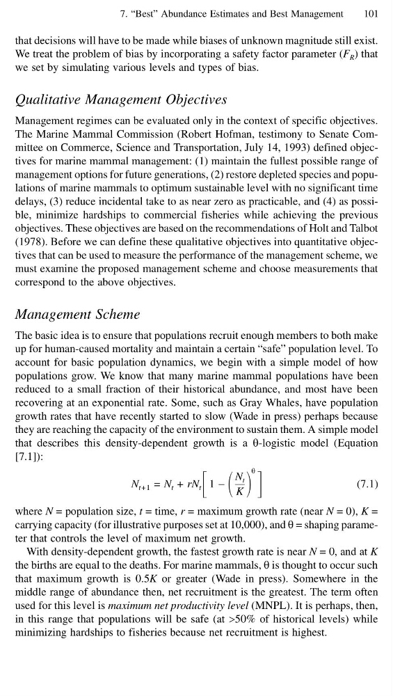
that describes this density-dependent growth is a θ-logistic model (Equation
[7.1]):
N t +1 = N t + rN t ΄ 1 −
N t
K
θ ΅
(7.1)
where N = population size, t = time, r = maximum growth rate (near N = 0), K =
carrying capacity (for illustrative purposes set at 10,000), and θ = shaping parameter that controls the level of maximum net growth.
With density-dependent growth, the fastest growth rate is near N = 0, and at K
the births are equal to the deaths. For marine mammals, θ is thought to occur such
that maximum growth is 0.5K or greater (Wade in press). Somewhere in the
middle range of abundance then, net recruitment is the greatest. The term often
used for this level is maximum net productivity level (MNPL). It is perhaps, then,
in this range that populations will be safe (at >50% of historical levels) while
minimizing hardships to fisheries because net recruitment is highest.
101
that decisions will have to be made while biases of unknown magnitude still exist.
We treat the problem of bias by incorporating a safety factor parameter (F R ) that
we set by simulating various levels and types of bias.
Qualitative Management Objectives
Management regimes can be evaluated only in the context of specific objectives.
The Marine Mammal Commission (Robert Hofman, testimony to Senate Committee on Commerce, Science and Transportation, July 14, 1993) defined objectives for marine mammal management: (1) maintain the fullest possible range of
management options for future generations, (2) restore depleted species and populations of marine mammals to optimum sustainable level with no significant time
delays, (3) reduce incidental take to as near zero as practicable, and (4) as possible, minimize hardships to commercial fisheries while achieving the previous
objectives. These objectives are based on the recommendations of Holt and Talbot
(1978). Before we can define these qualitative objectives into quantitative objectives that can be used to measure the performance of the management scheme, we
must examine the proposed management scheme and choose measurements that
correspond to the above objectives.
Management Scheme
The basic idea is to ensure that populations recruit enough members to both make
up for human-caused mortality and maintain a certain “safe” population level. To
account for basic population dynamics, we begin with a simple model of how
populations grow. We know that many marine mammal populations have been
reduced to a small fraction of their historical abundance, and most have been
recovering at an exponential rate. Some, such as Gray Whales, have population
growth rates that have recently started to slow (Wade in press) perhaps because
they are reaching the capacity of the environment to sustain them. A simple model
that describes this density-dependent growth is a θ-logistic model (Equation
[7.1]):
N t +1 = N t + rN t ΄ 1 −
N t
K
θ ΅
(7.1)
where N = population size, t = time, r = maximum growth rate (near N = 0), K =
carrying capacity (for illustrative purposes set at 10,000), and θ = shaping parameter that controls the level of maximum net growth.
With density-dependent growth, the fastest growth rate is near N = 0, and at K
the births are equal to the deaths. For marine mammals, θ is thought to occur such
that maximum growth is 0.5K or greater (Wade in press). Somewhere in the
middle range of abundance then, net recruitment is the greatest. The term often
used for this level is maximum net productivity level (MNPL). It is perhaps, then,
in this range that populations will be safe (at >50% of historical levels) while
minimizing hardships to fisheries because net recruitment is highest.