

100
Barbara L. Taylor and Paul R. Wade
After conducting a survey, we do not have the distributions shown in Figure
7.3b. Instead, we have an abundance estimate (N MEAN ) and an estimate of the
precision of our survey. For illustration, consider the case in which both Blue and
Beaked Whales are estimated to number 1,200, with CVs of 0.2 and 0.8, respectively. Because N MEAN is the same, both populations would be treated the same
under the N MEAN strategy. To incorporate uncertainty in our estimate into management, we need to focus on the tails of the distribution rather than on the measure of
central tendency (the mean or best estimate), which is the same for both distributions. Take, for example, the abundance estimate for which 95% of all abundance
estimates will be greater. For A this value is 867, whereas for B it is 371 (Fig.
7.3b). The mean or best estimate is the only point of similarity between these
distributions. If we want to give importance to the difference in our degree of
certainty, we should consider something other than the mean. The actual percentage of the distribution chosen depends on our management objectives. A sample
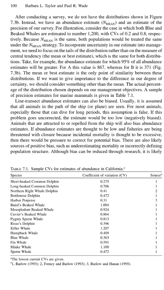
of precision estimates for marine mammals is given in Table 7.1.
Line-transect abundance estimates can also be biased. Usually, it is assumed
that all animals in the path of the ship (or plane) are seen. For most animals,
especially those that can dive for long periods, this assumption is false. If this
problem goes uncorrected, the estimate would be too low (negatively biased).
Animals that are attracted to or repelled from the ship will also bias abundance
estimates. If abundance estimates are thought to be low and fisheries are being
threatened with closure because incidental mortality is thought to be excessive,
then there would be pressure to correct for potential bias. There are also likely
sources of positive bias, such as underestimating mortality or incorrectly defining
population structure. Although bias can be reduced through research, it is likely
Table 7.1. Sample CVs for estimates of abundance in California.
a
Species
Coefficient of variation (CV)
Source
b
Short-beaked Common Dolphin
0.275
1
Long-beaked Common Dolphin
0.706
1
Northern Right Whale Dolphin
0.41
2
Bottlenose Dolphin
0.472
1
Harbor Porpoise
0.31
3
Baird’s Beaked Whale
1.004
1
Mesoplodont Beaked Whale
0.924
1
Cuvier’s Beaked Whale
0.864
1
Pygmy Sperm Whale
0.813
1
Risso’s Dolphin
0.396
1
Killer Whale
1.207
1
Humpback Whale
0.409
1
Blue Whale
0.363
1
Fin Whale
0.591
1
Minke Whale
1.100
1
Sperm Whale
0.472
1
a
The lowest current CVs are given.
b
1, Barlow (1993); 2, Forney and Barlow (1993); 3, Barlow and Hanan (1995).
Barbara L. Taylor and Paul R. Wade
After conducting a survey, we do not have the distributions shown in Figure
7.3b. Instead, we have an abundance estimate (N MEAN ) and an estimate of the
precision of our survey. For illustration, consider the case in which both Blue and
Beaked Whales are estimated to number 1,200, with CVs of 0.2 and 0.8, respectively. Because N MEAN is the same, both populations would be treated the same
under the N MEAN strategy. To incorporate uncertainty in our estimate into management, we need to focus on the tails of the distribution rather than on the measure of
central tendency (the mean or best estimate), which is the same for both distributions. Take, for example, the abundance estimate for which 95% of all abundance
estimates will be greater. For A this value is 867, whereas for B it is 371 (Fig.
7.3b). The mean or best estimate is the only point of similarity between these
distributions. If we want to give importance to the difference in our degree of
certainty, we should consider something other than the mean. The actual percentage of the distribution chosen depends on our management objectives. A sample
of precision estimates for marine mammals is given in Table 7.1.
Line-transect abundance estimates can also be biased. Usually, it is assumed
that all animals in the path of the ship (or plane) are seen. For most animals,
especially those that can dive for long periods, this assumption is false. If this
problem goes uncorrected, the estimate would be too low (negatively biased).
Animals that are attracted to or repelled from the ship will also bias abundance
estimates. If abundance estimates are thought to be low and fisheries are being
threatened with closure because incidental mortality is thought to be excessive,
then there would be pressure to correct for potential bias. There are also likely
sources of positive bias, such as underestimating mortality or incorrectly defining
population structure. Although bias can be reduced through research, it is likely
Table 7.1. Sample CVs for estimates of abundance in California.
a
Species
Coefficient of variation (CV)
Source
b
Short-beaked Common Dolphin
0.275
1
Long-beaked Common Dolphin
0.706
1
Northern Right Whale Dolphin
0.41
2
Bottlenose Dolphin
0.472
1
Harbor Porpoise
0.31
3
Baird’s Beaked Whale
1.004
1
Mesoplodont Beaked Whale
0.924
1
Cuvier’s Beaked Whale
0.864
1
Pygmy Sperm Whale
0.813
1
Risso’s Dolphin
0.396
1
Killer Whale
1.207
1
Humpback Whale
0.409
1
Blue Whale
0.363
1
Fin Whale
0.591
1
Minke Whale
1.100
1
Sperm Whale
0.472
1
a
The lowest current CVs are given.
b
1, Barlow (1993); 2, Forney and Barlow (1993); 3, Barlow and Hanan (1995).