

92
Michael J. Firko and Edward V. Podleckis
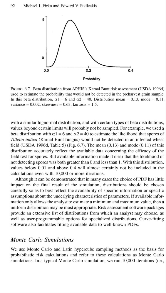
Figure 6.7. Beta distribution from APHIS’s Karnal Bunt risk assessment (USDA 1996d)
used to estimate the probability that would not be detected in the preharvest grain sample.
In this beta distribution, α1 = 6 and α2 = 40. Distribution mean = 0.13, mode = 0.11,
variance = 0.002, skewness = 0.63, kurtosis = 1.5.
with a similar lognormal distribution, and with certain types of beta distributions,
values beyond certain limits will probably not be sampled. For example, we used a
beta distribution with α1 = 6 and α2 = 40 to estimate the likelihood that spores of
Tilletia indica (Karnal Bunt fungus) would not be detected in an infected wheat
field (USDA 1996d, Table 5) (Fig. 6.7). The mean (0.13) and mode (0.11) of this
distribution accurately reflect the available data concerning the efficacy of the
field test for spores. But available information made it clear that the likelihood of
not detecting spores was both greater than 0 and less than 1. With this distribution,
values below 0.01 and above 0.4 will almost certainly not be included in the
calculations even with 10,000 or more iterations.
Although it can be demonstrated that in many cases the choice of PDF has little
impact on the final result of the simulation, distributions should be chosen
carefully so as to best reflect the availability of specific information or specific
assumptions about the underlying characteristics of parameters. If available information only allows the analyst to estimate a minimum and maximum value, then a
uniform distribution may be most appropriate. Risk assessment software packages
provide an extensive list of distributions from which an analyst may choose, as
well as user-programmable options for specialized distributions. Curve-fitting
software also facilitates fitting available data to well-known PDFs.
Monte Carlo Simulations
We use Monte Carlo and Latin hypercube sampling methods as the basis for
probabilistic risk calculations and refer to these calculations as Monte Carlo
simulations. In a typical Monte Carlo simulation, we run 10,000 iterations (i.e.,
Michael J. Firko and Edward V. Podleckis
Figure 6.7. Beta distribution from APHIS’s Karnal Bunt risk assessment (USDA 1996d)
used to estimate the probability that would not be detected in the preharvest grain sample.
In this beta distribution, α1 = 6 and α2 = 40. Distribution mean = 0.13, mode = 0.11,
variance = 0.002, skewness = 0.63, kurtosis = 1.5.
with a similar lognormal distribution, and with certain types of beta distributions,
values beyond certain limits will probably not be sampled. For example, we used a
beta distribution with α1 = 6 and α2 = 40 to estimate the likelihood that spores of
Tilletia indica (Karnal Bunt fungus) would not be detected in an infected wheat
field (USDA 1996d, Table 5) (Fig. 6.7). The mean (0.13) and mode (0.11) of this
distribution accurately reflect the available data concerning the efficacy of the
field test for spores. But available information made it clear that the likelihood of
not detecting spores was both greater than 0 and less than 1. With this distribution,
values below 0.01 and above 0.4 will almost certainly not be included in the
calculations even with 10,000 or more iterations.
Although it can be demonstrated that in many cases the choice of PDF has little
impact on the final result of the simulation, distributions should be chosen
carefully so as to best reflect the availability of specific information or specific
assumptions about the underlying characteristics of parameters. If available information only allows the analyst to estimate a minimum and maximum value, then a
uniform distribution may be most appropriate. Risk assessment software packages
provide an extensive list of distributions from which an analyst may choose, as
well as user-programmable options for specialized distributions. Curve-fitting
software also facilitates fitting available data to well-known PDFs.
Monte Carlo Simulations
We use Monte Carlo and Latin hypercube sampling methods as the basis for
probabilistic risk calculations and refer to these calculations as Monte Carlo
simulations. In a typical Monte Carlo simulation, we run 10,000 iterations (i.e.,