

Icebergs in the North Atlantic . ..
65
surrounding water (Russel-Head 1980). Therefore the heat exchange at the iceberg top is neglected, too.
In the current implementation, icebergs of predefined height h and radius r
(Fig. 1) are released at prescribed locations at fixed time intervals. Once an
iceberg has been generated, its drift and decay are computed as follows. First,
the horizontal velocities are averaged from the model grid over the total iceberg height (Fig. 1, shaded boxes to the left) to the current location of the
iceberg. The new position of the iceberg is then calculated by
( A) new (A) old .
180
(u cos ¢Old)
=
+ tIme step x
,
¢
¢
n Earth radius
ii
(1)
where A and ¢ denote longitude and latitude, respectively, and the averaged
zonal and meridional velocities are denoted by U and ii. We favour this Lagrangian approach because it more clearly reveals how the ocean might respond to
swarms of individual icebergs compared with an Eulerian technique. The latter
would have to be implemented in a fashion similar to one of the commonly
used sea-ice models, using some measure of iceberg coverage as a tracer. This
would require a high diffusion to maintain numerical stability, which can be
expected to broaden the iceberg drift paths and to yield results closer to those
obtained with pure meltwater inputs.
Like 11. and ii, the average temperature l' at the iceberg position is computed
from the surrounding model grid points, thus yielding the iceberg's melt rate
JL by the empirical relation from tank experiments:
JL = 0.018 (1' + l.8)l.5
(2)
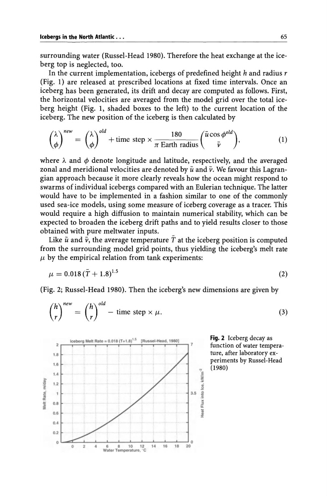
(Fig. 2; Russel-Head 1980). Then the iceberg's new dimensions are given by
( h) new (h) old
r
r
- time step x JL.
Icoberg Melt R.,. _ 0,018 (T+l .8)1.5 [Au ••• ,.H •• d , 19801
1.8
1.6
1.4
'"
..
~
1.2
!
o.s
::l
0 ,6
0,4
0.2
0
o
6
8
10
12
14
16
18
Water Temperature, C
"1
~
...
~
3 .5 2
.5
M
~
ii:
i
:z:
(3)
Fig. 2 Iceberg decay as
function of water temperature, after laboratory experiments by Russel-Head
(1980)
65
surrounding water (Russel-Head 1980). Therefore the heat exchange at the iceberg top is neglected, too.
In the current implementation, icebergs of predefined height h and radius r
(Fig. 1) are released at prescribed locations at fixed time intervals. Once an
iceberg has been generated, its drift and decay are computed as follows. First,
the horizontal velocities are averaged from the model grid over the total iceberg height (Fig. 1, shaded boxes to the left) to the current location of the
iceberg. The new position of the iceberg is then calculated by
( A) new (A) old .
180
(u cos ¢Old)
=
+ tIme step x
,
¢
¢
n Earth radius
ii
(1)
where A and ¢ denote longitude and latitude, respectively, and the averaged
zonal and meridional velocities are denoted by U and ii. We favour this Lagrangian approach because it more clearly reveals how the ocean might respond to
swarms of individual icebergs compared with an Eulerian technique. The latter
would have to be implemented in a fashion similar to one of the commonly
used sea-ice models, using some measure of iceberg coverage as a tracer. This
would require a high diffusion to maintain numerical stability, which can be
expected to broaden the iceberg drift paths and to yield results closer to those
obtained with pure meltwater inputs.
Like 11. and ii, the average temperature l' at the iceberg position is computed
from the surrounding model grid points, thus yielding the iceberg's melt rate
JL by the empirical relation from tank experiments:
JL = 0.018 (1' + l.8)l.5
(2)
(Fig. 2; Russel-Head 1980). Then the iceberg's new dimensions are given by
( h) new (h) old
r
r
- time step x JL.
Icoberg Melt R.,. _ 0,018 (T+l .8)1.5 [Au ••• ,.H •• d , 19801
1.8
1.6
1.4
'"
..
~
1.2
!
o.s
::l
0 ,6
0,4
0.2
0
o
6
8
10
12
14
16
18
Water Temperature, C
"1
~
...
~
3 .5 2
.5
M
~
ii:
i
:z:
(3)
Fig. 2 Iceberg decay as
function of water temperature, after laboratory experiments by Russel-Head
(1980)