

Model Simulation ofTemporal Variability of Suspended Matter in the North Sea
55
following, the computed SPM concentrations will be regarded only. Finally, the
result for the computed data will be assumed to be also valid for the measured
data.
S.l
Time Representativity
Question no. 1 is answered as follows: for each NSP station (with more than one
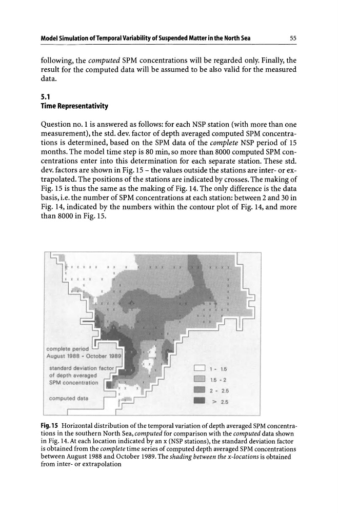
measurement), the std. dev. factor of depth averaged computed SPM concentrations is determined, based on the SPM data of the complete NSP period of 15
months. The model time step is 80 min, so more than 8000 computed SPM concentrations enter into this determination for each separate station. These std.
dev. factors are shown in Fig. 15 - the values outside the stations are inter- or extrapolated. The positions of the stations are indicated by crosses. The making of
Fig. 15 is thus the same as the making of Fig. 14. The only difference is the data
basis, i.e. the number of SPM concentrations at each station: between 2 and 30 in
Fig. 14, indicated by the numbers within the contour plot of Fig. 14, and more
than 8000 in Fig. 15.
standard deviation factor
D 1 - 1.6
of depth avaragad
D 16 - 2
SPM concentration
-
2 - 2.5
computed data
-
> 2.6
Fig.1S Horizontal distribution of the temporal variation of depth averaged SPM concentrations in the southern North Sea, computed for comparison with the computed data shown
in Fig. 14. At each location indicated by an x (NSP stations), the standard deviation factor
is obtained from the complete time series of computed depth averaged SPM concentrations
between August 1988 and October 1989. The shading between the x-locations is obtained
from inter- or extrapolation
55
following, the computed SPM concentrations will be regarded only. Finally, the
result for the computed data will be assumed to be also valid for the measured
data.
S.l
Time Representativity
Question no. 1 is answered as follows: for each NSP station (with more than one
measurement), the std. dev. factor of depth averaged computed SPM concentrations is determined, based on the SPM data of the complete NSP period of 15
months. The model time step is 80 min, so more than 8000 computed SPM concentrations enter into this determination for each separate station. These std.
dev. factors are shown in Fig. 15 - the values outside the stations are inter- or extrapolated. The positions of the stations are indicated by crosses. The making of
Fig. 15 is thus the same as the making of Fig. 14. The only difference is the data
basis, i.e. the number of SPM concentrations at each station: between 2 and 30 in
Fig. 14, indicated by the numbers within the contour plot of Fig. 14, and more
than 8000 in Fig. 15.
standard deviation factor
D 1 - 1.6
of depth avaragad
D 16 - 2
SPM concentration
-
2 - 2.5
computed data
-
> 2.6
Fig.1S Horizontal distribution of the temporal variation of depth averaged SPM concentrations in the southern North Sea, computed for comparison with the computed data shown
in Fig. 14. At each location indicated by an x (NSP stations), the standard deviation factor
is obtained from the complete time series of computed depth averaged SPM concentrations
between August 1988 and October 1989. The shading between the x-locations is obtained
from inter- or extrapolation