

56
w. Puis· T. Pohlmann· J. Stindermann
The comparison of Figs. 14 and 15 shows: the two patterns of std. dev. factors
are nearly identical. Only in the Dogger Bank area, the temporal variability was
insufficiently registered by the NSP cruises. The spatial means are 1.74 and 1.89
in Figs. 14 and 15, respectively. Answering question no. 1, it is concluded that,
with regard to the temporal variation of depth averaged SPM concentrations, the
frequency of NSP survey cruises was sufficient to yield a representative picture
of the complete NSP period August 1988-0ctober 1989.
5.2
Space Representativity
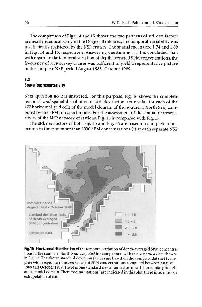
Next, question no. 2 is answered. For this purpose, Fig. 16 shows the complete
temporal and spatial distribution of std. dev. factors (one value for each of the
477 horizontal grid cells of the model domain of the southern North Sea) computed by the SPM transport model. For the assessment of the spatial representativity of the NSP network of stations, Fig. 16 is compared with Fig. 15.
The std. dev. factors of both Fig. 15 and Fig. 16 are based on complete information in time: on more than 8000 SPM concentrations (i) at each separate NSP
standard daviation factor
0 1 - 16
of depth aver8ged
CJ 1.5 - 2
SPM concentr8tion
2 - 2.5
computed data
-
> 2.5
Fig.16 Horizontal distribution of the temporal variation of depth -averaged SPM con centra -
tions in the southern North Sea, computed for comparison with the computed data shown
in Fig. 15. The shown standard deviation factors are based on the complete data set (complete with respect to time and space) of SPM concentrations computed between August
1988 and October 1989. There is one standard deviation factor at each horizontal grid cell
of the model domain. Therefore, no "stations" are indicated in this plot, there is no inter- or
extrapolation of data
w. Puis· T. Pohlmann· J. Stindermann
The comparison of Figs. 14 and 15 shows: the two patterns of std. dev. factors
are nearly identical. Only in the Dogger Bank area, the temporal variability was
insufficiently registered by the NSP cruises. The spatial means are 1.74 and 1.89
in Figs. 14 and 15, respectively. Answering question no. 1, it is concluded that,
with regard to the temporal variation of depth averaged SPM concentrations, the
frequency of NSP survey cruises was sufficient to yield a representative picture
of the complete NSP period August 1988-0ctober 1989.
5.2
Space Representativity
Next, question no. 2 is answered. For this purpose, Fig. 16 shows the complete
temporal and spatial distribution of std. dev. factors (one value for each of the
477 horizontal grid cells of the model domain of the southern North Sea) computed by the SPM transport model. For the assessment of the spatial representativity of the NSP network of stations, Fig. 16 is compared with Fig. 15.
The std. dev. factors of both Fig. 15 and Fig. 16 are based on complete information in time: on more than 8000 SPM concentrations (i) at each separate NSP
standard daviation factor
0 1 - 16
of depth aver8ged
CJ 1.5 - 2
SPM concentr8tion
2 - 2.5
computed data
-
> 2.5
Fig.16 Horizontal distribution of the temporal variation of depth -averaged SPM con centra -
tions in the southern North Sea, computed for comparison with the computed data shown
in Fig. 15. The shown standard deviation factors are based on the complete data set (complete with respect to time and space) of SPM concentrations computed between August
1988 and October 1989. There is one standard deviation factor at each horizontal grid cell
of the model domain. Therefore, no "stations" are indicated in this plot, there is no inter- or
extrapolation of data