

Methods Used in a Mass-Balance Study of Holocene Sediment Accumulation on the ...
367
these constructions, for instance, isolated sites at which the base of the Holocene
was encountered in an unusually deep position in a borehole may be interpreted
as belonging to a narrow gully. By attributing an isolated point to an extensive
gully system, however, an individual depth value receives a new and wider spatial significance. Digitizing of the contour lines produced a large number of
points arranged along these lines, comprising a very high data density. For the
purpose of the study, these scattered data had to be transformed into a regular
grid.
Compared with manual construction, computer programs make exclusive
use of borehole data regardless of geological or morphogenetic aspects. The
scattered depth values obtained from borehole records are transposed directly
onto a regular grid, which is most suitable for volume determinations.
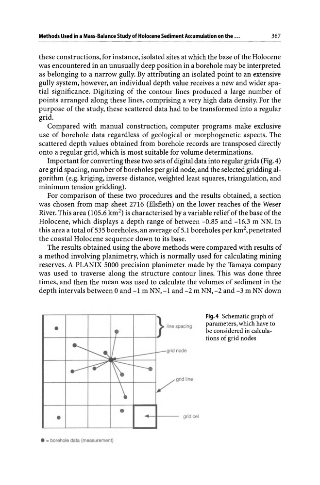
Important for converting these two sets of digital data into regular grids (Fig. 4)
are grid spacing, number of boreholes per grid node, and the selected gridding algorithm (e.g. kriging, inverse distance, weighted least squares, triangulation, and
minimum tension gridding).
For comparison of these two procedures and the results obtained, a section
was chosen from map sheet 2716 (Elsfleth) on the lower reaches of the Weser
River. This area (105.6 km 2 ) is characterised by a variable relief of the base of the
Holocene, which displays a depth range of between -0.85 and -16.3 m NN. In
this area a total of 535 boreholes, an average of 5.1 boreholes per km 2 , penetrated
the coastal Holocene sequence down to its base.
The results obtained using the above methods were compared with results of
a method involving planimetry, which is normally used for calculating mining
reserves. A PLANIX 5000 precision planimeter made by the Tamaya company
was used to traverse along the structure contour lines. This was done three
times, and then the mean was used to calculate the volumes of sediment in the
depth intervals between 0 and -1 m NN, -1 and -2 m NN, -2 and -3 m NN down
I-_ e_ .-_---II--_---I-+-_--+ __ --i ,} line spacing
grid node
grid line
•
•
grid cel
• • borehole date (measurement)
Fig.4 Schematic graph of
parameters, which have to
be considered in calculations of grid nodes
367
these constructions, for instance, isolated sites at which the base of the Holocene
was encountered in an unusually deep position in a borehole may be interpreted
as belonging to a narrow gully. By attributing an isolated point to an extensive
gully system, however, an individual depth value receives a new and wider spatial significance. Digitizing of the contour lines produced a large number of
points arranged along these lines, comprising a very high data density. For the
purpose of the study, these scattered data had to be transformed into a regular
grid.
Compared with manual construction, computer programs make exclusive
use of borehole data regardless of geological or morphogenetic aspects. The
scattered depth values obtained from borehole records are transposed directly
onto a regular grid, which is most suitable for volume determinations.
Important for converting these two sets of digital data into regular grids (Fig. 4)
are grid spacing, number of boreholes per grid node, and the selected gridding algorithm (e.g. kriging, inverse distance, weighted least squares, triangulation, and
minimum tension gridding).
For comparison of these two procedures and the results obtained, a section
was chosen from map sheet 2716 (Elsfleth) on the lower reaches of the Weser
River. This area (105.6 km 2 ) is characterised by a variable relief of the base of the
Holocene, which displays a depth range of between -0.85 and -16.3 m NN. In
this area a total of 535 boreholes, an average of 5.1 boreholes per km 2 , penetrated
the coastal Holocene sequence down to its base.
The results obtained using the above methods were compared with results of
a method involving planimetry, which is normally used for calculating mining
reserves. A PLANIX 5000 precision planimeter made by the Tamaya company
was used to traverse along the structure contour lines. This was done three
times, and then the mean was used to calculate the volumes of sediment in the
depth intervals between 0 and -1 m NN, -1 and -2 m NN, -2 and -3 m NN down
I-_ e_ .-_---II--_---I-+-_--+ __ --i ,} line spacing
grid node
grid line
•
•
grid cel
• • borehole date (measurement)
Fig.4 Schematic graph of
parameters, which have to
be considered in calculations of grid nodes