

Milankovitch Cycles and Sequences: Two Different Stratigraphic Tools
2
to
::e 1
- .<: '& c:
.S!
CD
"0 0
'"
0
'0
CD
C>
c:
1-1
(,)
-2
0
2
4
6
8
10
Length of 3rd order sequence cycles (Mal
249
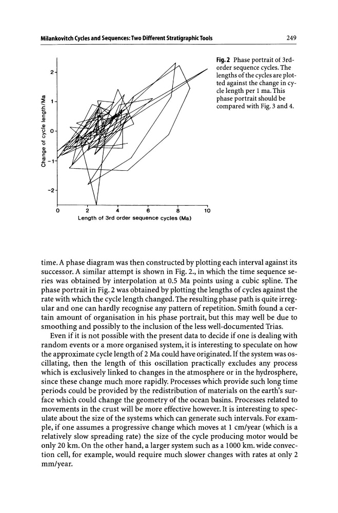
Fig.2 Phase portrait of 3rdorder sequence cycles. The
lengths of the cycles are plotted against the change in cycle length per 1 rna. This
phase portrait should be
compared with Fig. 3 and 4.
time. A phase diagram was then constructed by plotting each interval against its
successor. A similar attempt is shown in Fig. 2., in which the time sequence series was obtained by interpolation at 0.5 Ma points using a cubic spline. The
phase portrait in Fig. 2 was obtained by plotting the lengths of cycles against the
rate with which the cycle length changed. The resulting phase path is quite irregular and one can hardly recognise any pattern of repetition. Smith found a certain amount of organisation in his phase portrait, but this may well be due to
smoothing and possibly to the inclusion of the less well-documented Trias.
Even if it is not possible with the present data to decide if one is dealing with
random events or a more organised system, it is interesting to speculate on how
the approximate cycle length of 2 Ma could have originated. If the system was oscillating, then the length of this oscillation practically excludes any process
which is exclusively linked to changes in the atmosphere or in the hydrosphere,
since these change much more rapidly. Processes which provide such long time
periods could be provided by the redistribution of materials on the earth's surface which could change the geometry of the ocean basins. Processes related to
movements in the crust will be more effective however. It is interesting to speculate about the size of the systems which can generate such intervals. For example, if one assumes a progressive change which moves at 1 cm/year (which is a
relatively slow spreading rate) the size of the cycle producing motor would be
only 20 km. On the other hand, a larger system such as a 1000 km. wide convection cell, for example, would require much slower changes with rates at only 2
mm/year.
2
to
::e 1
- .<: '& c:
.S!
CD
"0 0
'"
0
'0
CD
C>
c:
1-1
(,)
-2
0
2
4
6
8
10
Length of 3rd order sequence cycles (Mal
249
Fig.2 Phase portrait of 3rdorder sequence cycles. The
lengths of the cycles are plotted against the change in cycle length per 1 rna. This
phase portrait should be
compared with Fig. 3 and 4.
time. A phase diagram was then constructed by plotting each interval against its
successor. A similar attempt is shown in Fig. 2., in which the time sequence series was obtained by interpolation at 0.5 Ma points using a cubic spline. The
phase portrait in Fig. 2 was obtained by plotting the lengths of cycles against the
rate with which the cycle length changed. The resulting phase path is quite irregular and one can hardly recognise any pattern of repetition. Smith found a certain amount of organisation in his phase portrait, but this may well be due to
smoothing and possibly to the inclusion of the less well-documented Trias.
Even if it is not possible with the present data to decide if one is dealing with
random events or a more organised system, it is interesting to speculate on how
the approximate cycle length of 2 Ma could have originated. If the system was oscillating, then the length of this oscillation practically excludes any process
which is exclusively linked to changes in the atmosphere or in the hydrosphere,
since these change much more rapidly. Processes which provide such long time
periods could be provided by the redistribution of materials on the earth's surface which could change the geometry of the ocean basins. Processes related to
movements in the crust will be more effective however. It is interesting to speculate about the size of the systems which can generate such intervals. For example, if one assumes a progressive change which moves at 1 cm/year (which is a
relatively slow spreading rate) the size of the cycle producing motor would be
only 20 km. On the other hand, a larger system such as a 1000 km. wide convection cell, for example, would require much slower changes with rates at only 2
mm/year.