

134
B. J. Haupt· K. Stattegger . D. Seidov
a)
cl
8
2:
Fig.1Sa,b Modern velocity:
z
z
~
il
a at z=25 m and b at the
90'"
bottom. The bottom veloci"'F
ty in the I-em-thick bottom
~'"
is smoothed with a sliding
average with ten passes
"til'"
-b.",
.;;~
~'"
.t>"
4>~
oj$'"
"0"
l
~
~
~
~
0.
'&
~
io
~
..
..
b)
i'\
I!:.
";
z
z
grrw
"'f
!Ii'"
i'
"til'"
-b.",
"
4>~
oj$'"
"
~ •
•
' •
l
.. .. ...... .. ~ . .. ,
• • • • ~ r ..... . .
,
•
. . : .... ...
,~
~
~
"0,
'&
I?
io
~
..
'"
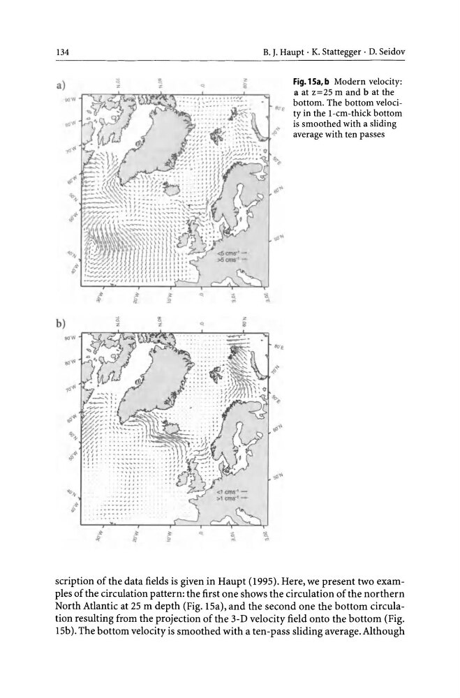
scription of the data fields is given in Haupt (1995). Here, we present two examples of the circulation pattern: the first one shows the circulation of the northern
North Atlantic at 25 m depth (Fig. I5a), and the second one the bottom circulation resulting from the projection of the 3-D velocity field onto the bottom (Fig.
I5b). The bottom velocity is smoothed with a ten-pass sliding average. Although
B. J. Haupt· K. Stattegger . D. Seidov
a)
cl
8
2:
Fig.1Sa,b Modern velocity:
z
z
~
il
a at z=25 m and b at the
90'"
bottom. The bottom veloci"'F
ty in the I-em-thick bottom
~'"
is smoothed with a sliding
average with ten passes
"til'"
-b.",
.;;~
~'"
.t>"
4>~
oj$'"
"0"
l
~
~
~
~
0.
'&
~
io
~
..
..
b)
i'\
I!:.
";
z
z
grrw
"'f
!Ii'"
i'
"til'"
-b.",
"
4>~
oj$'"
"
~ •
•
' •
l
.. .. ...... .. ~ . .. ,
• • • • ~ r ..... . .
,
•
. . : .... ...
,~
~
~
"0,
'&
I?
io
~
..
'"
scription of the data fields is given in Haupt (1995). Here, we present two examples of the circulation pattern: the first one shows the circulation of the northern
North Atlantic at 25 m depth (Fig. I5a), and the second one the bottom circulation resulting from the projection of the 3-D velocity field onto the bottom (Fig.
I5b). The bottom velocity is smoothed with a ten-pass sliding average. Although