

2 Identifying Ice Floes and Computing Ice Floe Distributions in SAR Images
23
Table 2. Floe bin size used in
time series study
No.
No. of Pixels
Maximum area
L(m)
(km')
0.01
123
2
2
0.02
174
3
3-4
0.Q4
256
4
5-8
0.08
348
5
9-16
0.16
492
6
17-64
0.64
985
7
65-256
2.56
1969
8
257-1600
16.0
4924
9
1601-6400
64.0
9847
10
>6400
>64.0
>9847
From Rothrock and Thorndike (1984). Area = axU, where a =
0.66 and L = mean diameter.
The algorithm procedures described in the previous sections were applied to ERS-1
C-band SAR imagery sampled down to about 225 m resolution (100 m pixel size) from
the finer resolution (25 m) original data. The output was separated into four classes as
described above: measurable floes, floes originally characterized by the algorithm as
floes but considered too branchy (labeled discarded), open water, and the remainder of
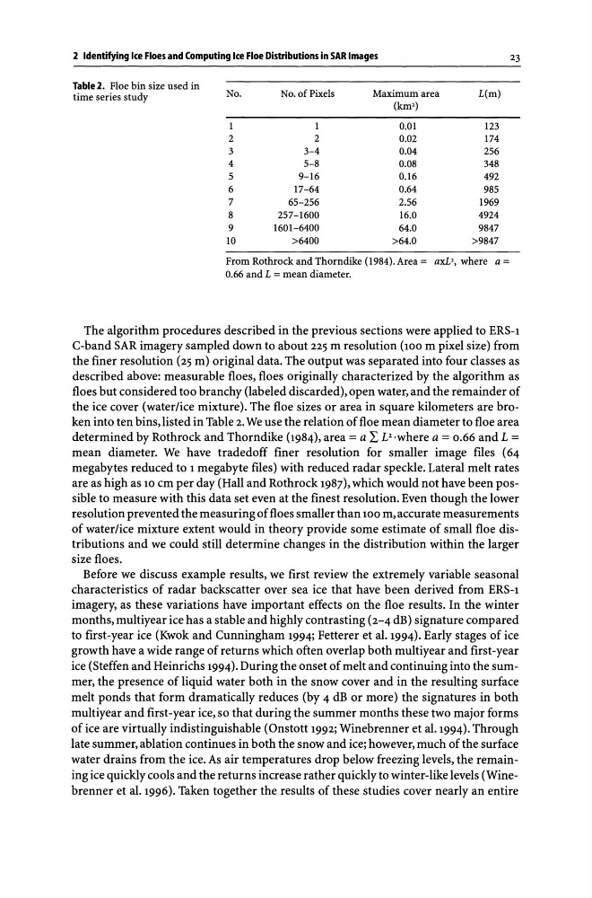
the ice cover (water/ice mixture). The floe sizes or area in square kilometers are broken into ten bins, listed in Table 2. We use the relation of floe mean diameter to floe area
determined by Rothrock and Thorndike (1984), area = a I. U 'where a = 0.66 and L =
mean diameter. We have tradedoff finer resolution for smaller image files (64
megabytes reduced to 1 megabyte files) with reduced radar speckle. Lateral melt rates
are as high as 10 cm per day (Hall and Rothrock 1987), which would not have been possible to measure with this data set even at the finest resolution. Even though the lower
resolution prevented the measuring of floes smaller than 100 m, accurate measurements
of water/ice mixture extent would in theory provide some estimate of small floe distributions and we could still determine changes in the distribution within the larger
size floes.
Before we discuss example results, we first review the extremely variable seasonal
characteristics of radar backscatter over sea ice that have been derived from ERS-1
imagery, as these variations have important effects on the floe results. In the winter
months, multiyear ice has a stable and highly contrasting (2-4 dB) signature compared
to first-year ice (Kwok and Cunningham 1994; Fetterer et al. 1994). Early stages of ice
growth have a wide range of returns which often overlap both multiyear and first-year
ice (Steffen and Heinrichs 1994). During the onset of melt and continuing into the summer, the presence of liquid water both in the snow cover and in the resulting surface
melt ponds that form dramatically reduces (by 4 dB or more) the signatures in both
multiyear and first-year ice, so that during the summer months these two major forms
of ice are virtually indistinguishable (Onstott 1992; Winebrenner et al. 1994). Through
late summer, ablation continues in both the snow and ice; however, much of the surface
water drains from the ice. As air temperatures drop below freezing levels, the remaining ice quickly cools and the returns increase rather quickly to winter-like levels (Winebrenner et al. 1996). Taken together the results of these studies cover nearly an entire
23
Table 2. Floe bin size used in
time series study
No.
No. of Pixels
Maximum area
L(m)
(km')
0.01
123
2
2
0.02
174
3
3-4
0.Q4
256
4
5-8
0.08
348
5
9-16
0.16
492
6
17-64
0.64
985
7
65-256
2.56
1969
8
257-1600
16.0
4924
9
1601-6400
64.0
9847
10
>6400
>64.0
>9847
From Rothrock and Thorndike (1984). Area = axU, where a =
0.66 and L = mean diameter.
The algorithm procedures described in the previous sections were applied to ERS-1
C-band SAR imagery sampled down to about 225 m resolution (100 m pixel size) from
the finer resolution (25 m) original data. The output was separated into four classes as
described above: measurable floes, floes originally characterized by the algorithm as
floes but considered too branchy (labeled discarded), open water, and the remainder of
the ice cover (water/ice mixture). The floe sizes or area in square kilometers are broken into ten bins, listed in Table 2. We use the relation of floe mean diameter to floe area
determined by Rothrock and Thorndike (1984), area = a I. U 'where a = 0.66 and L =
mean diameter. We have tradedoff finer resolution for smaller image files (64
megabytes reduced to 1 megabyte files) with reduced radar speckle. Lateral melt rates
are as high as 10 cm per day (Hall and Rothrock 1987), which would not have been possible to measure with this data set even at the finest resolution. Even though the lower
resolution prevented the measuring of floes smaller than 100 m, accurate measurements
of water/ice mixture extent would in theory provide some estimate of small floe distributions and we could still determine changes in the distribution within the larger
size floes.
Before we discuss example results, we first review the extremely variable seasonal
characteristics of radar backscatter over sea ice that have been derived from ERS-1
imagery, as these variations have important effects on the floe results. In the winter
months, multiyear ice has a stable and highly contrasting (2-4 dB) signature compared
to first-year ice (Kwok and Cunningham 1994; Fetterer et al. 1994). Early stages of ice
growth have a wide range of returns which often overlap both multiyear and first-year
ice (Steffen and Heinrichs 1994). During the onset of melt and continuing into the summer, the presence of liquid water both in the snow cover and in the resulting surface
melt ponds that form dramatically reduces (by 4 dB or more) the signatures in both
multiyear and first-year ice, so that during the summer months these two major forms
of ice are virtually indistinguishable (Onstott 1992; Winebrenner et al. 1994). Through
late summer, ablation continues in both the snow and ice; however, much of the surface
water drains from the ice. As air temperatures drop below freezing levels, the remaining ice quickly cools and the returns increase rather quickly to winter-like levels (Winebrenner et al. 1996). Taken together the results of these studies cover nearly an entire