

3.7 Numerical Integration of the Source Function
69
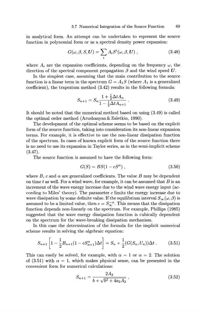
in analytical form. An attempt can be undertaken to represent the source
function in polynomial form or as a spectral density power expansion:
(3.48)
where Ai are the expansion coefficients, depending on the frequency w, the
direction of the spectral component propagation {3 and the wind speed U.
In the simplest case, assuming that the main contribution to the source
function is a linear term in the spectrum G = A 1 S (where A1 is a generalized
coefficient), the trapezium method (3.42) results in the following formula:
1 +~~tAn
Sn+l = Sn
1 ~ A
1- 2 t n+l
(3.49)
It should be noted that the numerical method based on using (3.49) is called
the optimal order method ( Arushanyan & Zaletkin, 1990).
The development of the optimal scheme seems to be based on the explicit
form of the source function, taking into consideration its non-linear expansion
terms. For example, it is effective to use the non-linear dissipation function
of the spectrum. In cases of known explicit form of the source function there
is no need to use its expansion in Taylor series, as in the semi-implicit scheme
(3.47).
The source function is assumed to have the following form:
G(S) = BS(1 - cS 0 ) ,
(3.50)
where B, c and a are generalized coefficients. The value B may be dependent
on timet as well. For a wind wave, for example, it can be assumed that B is an
increment of the wave energy increase due to the wind wave energy input ( according to Miles' theory). The parameter c limits the energy increase due to
wave dissipation by some definite value. If the equilibrium interval 800 (w, {3) is
assumed to be a limited value, then c = s;;,o:. This means that the dissipation
function depends non-linearly on the spectrum. For example, Phillips (1985)
suggested that the wave energy dissipation function is cubically dependent
on the spectrum for the wave-breaking dissipation mechanism.
In this case the determination of the formula for the implicit numerical
scheme results in solving the algebraic equation:
(3.51)
This can easily be solved, for example, with a = 1 or a = 2. The solution
of (3.51) with a = 1, which makes physical sense, can be presented in the
convenient form for numerical calculations:
(3.52)
69
in analytical form. An attempt can be undertaken to represent the source
function in polynomial form or as a spectral density power expansion:
(3.48)
where Ai are the expansion coefficients, depending on the frequency w, the
direction of the spectral component propagation {3 and the wind speed U.
In the simplest case, assuming that the main contribution to the source
function is a linear term in the spectrum G = A 1 S (where A1 is a generalized
coefficient), the trapezium method (3.42) results in the following formula:
1 +~~tAn
Sn+l = Sn
1 ~ A
1- 2 t n+l
(3.49)
It should be noted that the numerical method based on using (3.49) is called
the optimal order method ( Arushanyan & Zaletkin, 1990).
The development of the optimal scheme seems to be based on the explicit
form of the source function, taking into consideration its non-linear expansion
terms. For example, it is effective to use the non-linear dissipation function
of the spectrum. In cases of known explicit form of the source function there
is no need to use its expansion in Taylor series, as in the semi-implicit scheme
(3.47).
The source function is assumed to have the following form:
G(S) = BS(1 - cS 0 ) ,
(3.50)
where B, c and a are generalized coefficients. The value B may be dependent
on timet as well. For a wind wave, for example, it can be assumed that B is an
increment of the wave energy increase due to the wind wave energy input ( according to Miles' theory). The parameter c limits the energy increase due to
wave dissipation by some definite value. If the equilibrium interval 800 (w, {3) is
assumed to be a limited value, then c = s;;,o:. This means that the dissipation
function depends non-linearly on the spectrum. For example, Phillips (1985)
suggested that the wave energy dissipation function is cubically dependent
on the spectrum for the wave-breaking dissipation mechanism.
In this case the determination of the formula for the implicit numerical
scheme results in solving the algebraic equation:
(3.51)
This can easily be solved, for example, with a = 1 or a = 2. The solution
of (3.51) with a = 1, which makes physical sense, can be presented in the
convenient form for numerical calculations:
(3.52)