

62
3 Numerical Implementation of the Wave Energy Balance Equation
66.0
a)
61.0
56.0
lf{ b)
71.0 r0.25
:::::.:
0.75
::::
66.0~.25- - -
6f.O....._~ .........
_'::::--~~1.00
56.0 , ..... _ _ _ _ __;0..;:,50~7- _ _ _ _ _
Sf.Ot2"W9 6 J 0 J 6 9"E f2"W9 6 J 0 J 6 9"E
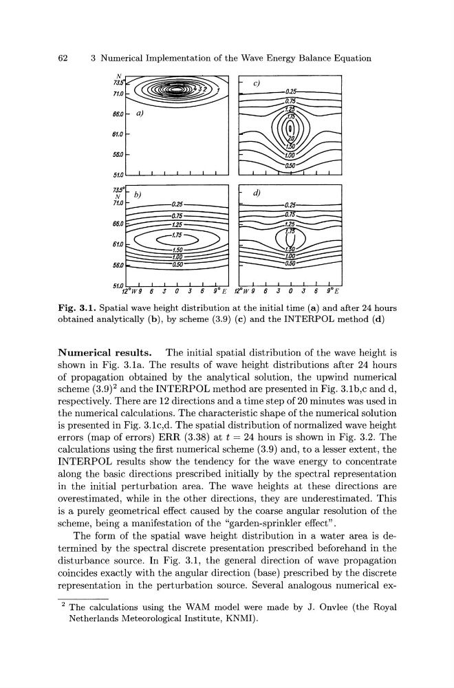
Fig. 3.1. Spatial wave height distribution at the initial time (a) and after 24 hours
obtained analytically (b), by scheme (3.9) (c) and the INTERPOL method (d)
Numerical results. The initial spatial distribution of the wave height is
shown in Fig. 3.1a. The results of wave height distributions after 24 hours
of propagation obtained by the analytical solution, the upwind numerical
scheme (3.9) 2 and the INTERPOL method are presented in Fig. 3.lb,c and d,
respectively. There are 12 directions and a time step of 20 minutes was used in
the numerical calculations. The characteristic shape of the numerical solution
is presented in Fig. 3.1c,d. The spatial distribution of normalized wave height
errors (map of errors) ERR (3.38) at t = 24 hours is shown in Fig. 3.2. The
calculations using the first numerical scheme (3.9) and, to a lesser extent, the
INTERPOL results show the tendency for the wave energy to concentrate
along the basic directions prescribed initially by the spectral representation
in the initial perturbation area. The wave heights at these directions are
overestimated, while in the other directions, they are underestimated. This
is a purely geometrical effect caused by the coarse angular resolution of the
scheme, being a manifestation of the "garden-sprinkler effect".
The form of the spatial wave height distribution in a water area is determined by the spectral discrete presentation prescribed beforehand in the
disturbance source. In Fig. 3.1, the general direction of wave propagation
coincides exactly with the angular direction (base) prescribed by the discrete
representation in the perturbation source. Several analogous numerical ex2 The calculations using the WAM model were made by J. Onvlee (the Royal
Netherlands Meteorological Institute, KNMI).
3 Numerical Implementation of the Wave Energy Balance Equation
66.0
a)
61.0
56.0
lf{ b)
71.0 r0.25
:::::.:
0.75
::::
66.0~.25- - -
6f.O....._~ .........
_'::::--~~1.00
56.0 , ..... _ _ _ _ __;0..;:,50~7- _ _ _ _ _
Sf.Ot2"W9 6 J 0 J 6 9"E f2"W9 6 J 0 J 6 9"E
Fig. 3.1. Spatial wave height distribution at the initial time (a) and after 24 hours
obtained analytically (b), by scheme (3.9) (c) and the INTERPOL method (d)
Numerical results. The initial spatial distribution of the wave height is
shown in Fig. 3.1a. The results of wave height distributions after 24 hours
of propagation obtained by the analytical solution, the upwind numerical
scheme (3.9) 2 and the INTERPOL method are presented in Fig. 3.lb,c and d,
respectively. There are 12 directions and a time step of 20 minutes was used in
the numerical calculations. The characteristic shape of the numerical solution
is presented in Fig. 3.1c,d. The spatial distribution of normalized wave height
errors (map of errors) ERR (3.38) at t = 24 hours is shown in Fig. 3.2. The
calculations using the first numerical scheme (3.9) and, to a lesser extent, the
INTERPOL results show the tendency for the wave energy to concentrate
along the basic directions prescribed initially by the spectral representation
in the initial perturbation area. The wave heights at these directions are
overestimated, while in the other directions, they are underestimated. This
is a purely geometrical effect caused by the coarse angular resolution of the
scheme, being a manifestation of the "garden-sprinkler effect".
The form of the spatial wave height distribution in a water area is determined by the spectral discrete presentation prescribed beforehand in the
disturbance source. In Fig. 3.1, the general direction of wave propagation
coincides exactly with the angular direction (base) prescribed by the discrete
representation in the perturbation source. Several analogous numerical ex2 The calculations using the WAM model were made by J. Onvlee (the Royal
Netherlands Meteorological Institute, KNMI).