

1.1 Hydrodynamic Problem of Surface Wave Generation by Air Flow
13
approximation U =grad(¢>). In this approximation the water motion can be
considered as potential and the dynamic equations for z < ry are as follows:
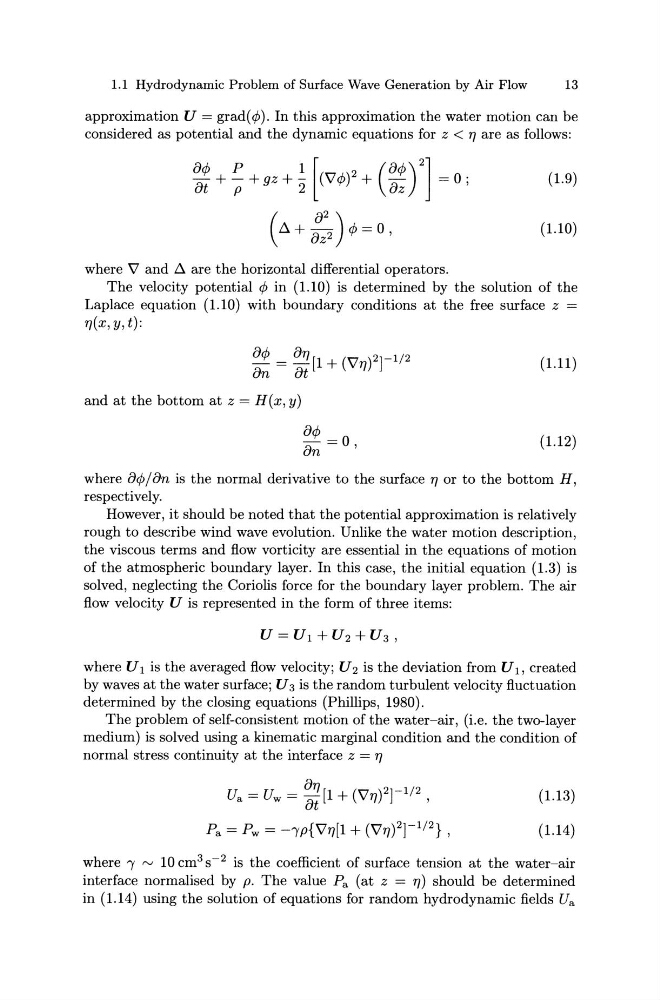
(1.9)
(1.10)
where \7 and ~ are the horizontal differential operators.
The velocity potential ¢> in (1.10) is determined by the solution of the
Laplace equation (1.10) with boundary conditions at the free surface z
ry(x, y, t):
(1.11)
and at the bottom at z = H(x, y)
8¢>
an =O'
(1.12)
where 8¢>j8n is the normal derivative to the surface ry or to the bottom H,
respectively.
However, it should be noted that the potential approximation is relatively
rough to describe wind wave evolution. Unlike the water motion description,
the viscous terms and flow vorticity are essential in the equations of motion
of the atmospheric boundary layer. In this case, the initial equation (1.3) is
solved, neglecting the Coriolis force for the boundary layer problem. The air
flow velocity U is represented in the form of three items:
where U 1 is the averaged flow velocity; U 2 is the deviation from U 1 , created
by waves at the water surface; U 3 is the random turbulent velocity fluctuation
determined by the closing equations (Phillips, 1980).
The problem of self-consistent motion of the water-air, (i.e. the two-layer
medium) is solved using a kinematic marginal condition and the condition of
normal stress continuity at the interface z = ry
Ua = Uw = ~~ [1 + ('Vry) 2 r 1 / 2 ,
Pa = Pw = -1'p{'V'ry[1 + ('Vry)2r1/2} '
(1.13)
(1.14)
where 1 rv 10 cm 3 s- 2 is the coefficient of surface tension at the water-air
interface normalised by p. The value Pa (at z = ry) should be determined
in (1.14) using the solution of equations for random hydrodynamic fields Ua
13
approximation U =grad(¢>). In this approximation the water motion can be
considered as potential and the dynamic equations for z < ry are as follows:
(1.9)
(1.10)
where \7 and ~ are the horizontal differential operators.
The velocity potential ¢> in (1.10) is determined by the solution of the
Laplace equation (1.10) with boundary conditions at the free surface z
ry(x, y, t):
(1.11)
and at the bottom at z = H(x, y)
8¢>
an =O'
(1.12)
where 8¢>j8n is the normal derivative to the surface ry or to the bottom H,
respectively.
However, it should be noted that the potential approximation is relatively
rough to describe wind wave evolution. Unlike the water motion description,
the viscous terms and flow vorticity are essential in the equations of motion
of the atmospheric boundary layer. In this case, the initial equation (1.3) is
solved, neglecting the Coriolis force for the boundary layer problem. The air
flow velocity U is represented in the form of three items:
where U 1 is the averaged flow velocity; U 2 is the deviation from U 1 , created
by waves at the water surface; U 3 is the random turbulent velocity fluctuation
determined by the closing equations (Phillips, 1980).
The problem of self-consistent motion of the water-air, (i.e. the two-layer
medium) is solved using a kinematic marginal condition and the condition of
normal stress continuity at the interface z = ry
Ua = Uw = ~~ [1 + ('Vry) 2 r 1 / 2 ,
Pa = Pw = -1'p{'V'ry[1 + ('Vry)2r1/2} '
(1.13)
(1.14)
where 1 rv 10 cm 3 s- 2 is the coefficient of surface tension at the water-air
interface normalised by p. The value Pa (at z = ry) should be determined
in (1.14) using the solution of equations for random hydrodynamic fields Ua