

5.4 Estimation of Non-Linear Wave Interaction in the Rip Spectrum
177
y V(X) a)
y
b)
-----8
c
8
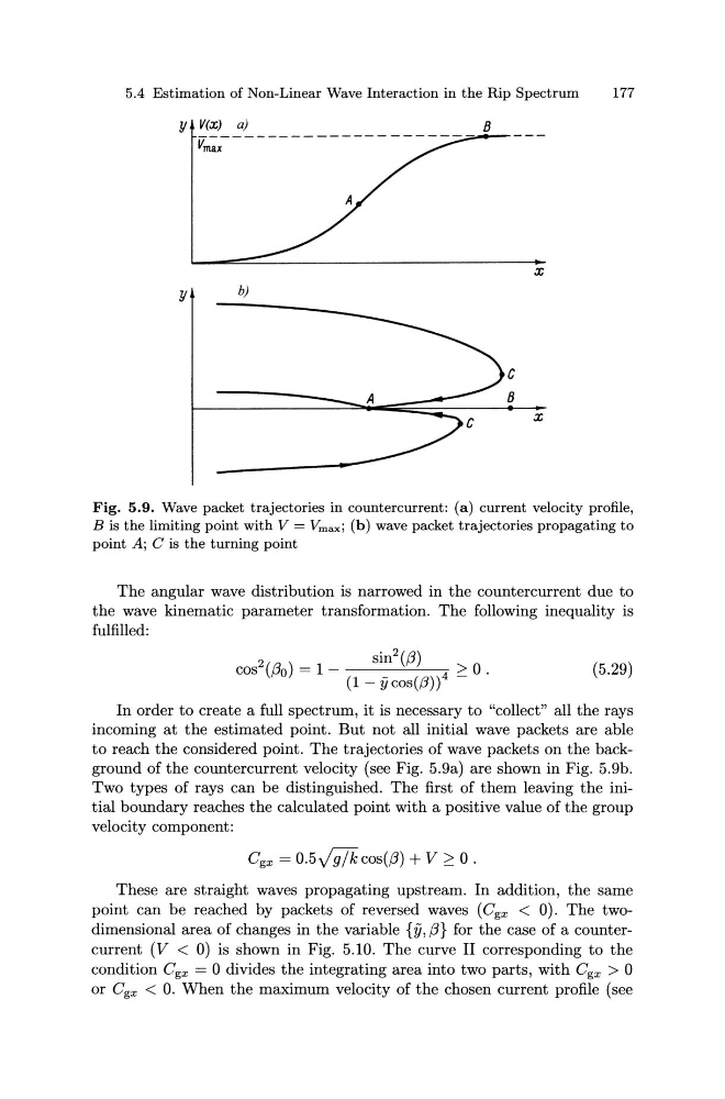
Fig. 5.9. Wave packet trajectories in countercurrent: (a) current velocity profile,
B is the limiting point with V = Vmaxi (b) wave packet trajectories propagating to
point A; C is the turning point
The angular wave distribution is narrowed in the countercurrent due to
the wave kinematic parameter transformation. The following inequality is
fulfilled:
2 ({3 ) 1
sin2 ({3)
cos 0 = -
4?:0.
(1- ycos(,6))
(5.29)
In order to create a full spectrum, it is necessary to "collect" all the rays
incoming at the estimated point. But not all initial wave packets are able
to reach the considered point. The trajectories of wave packets on the background of the countercurrent velocity (see Fig. 5.9a) are shown in Fig. 5.9b.
Two types of rays can be distinguished. The first of them leaving the initial boundary reaches the calculated point with a positive value of the group
velocity component:
Cgx = 0.5V9/kcos({J) + V?: 0.
These are straight waves propagating upstream. In addition, the same
point can be reached by packets of reversed waves (Cgx < 0). The twodimensional area of changes in the variable {y, {3} for the case of a countercurrent (V < 0) is shown in Fig. 5.10. The curve II corresponding to the
condition Cgx = 0 divides the integrating area into two parts, with Cgx > 0
or Cgx < 0. When the maximum velocity of the chosen current profile (see
177
y V(X) a)
y
b)
-----8
c
8
Fig. 5.9. Wave packet trajectories in countercurrent: (a) current velocity profile,
B is the limiting point with V = Vmaxi (b) wave packet trajectories propagating to
point A; C is the turning point
The angular wave distribution is narrowed in the countercurrent due to
the wave kinematic parameter transformation. The following inequality is
fulfilled:
2 ({3 ) 1
sin2 ({3)
cos 0 = -
4?:0.
(1- ycos(,6))
(5.29)
In order to create a full spectrum, it is necessary to "collect" all the rays
incoming at the estimated point. But not all initial wave packets are able
to reach the considered point. The trajectories of wave packets on the background of the countercurrent velocity (see Fig. 5.9a) are shown in Fig. 5.9b.
Two types of rays can be distinguished. The first of them leaving the initial boundary reaches the calculated point with a positive value of the group
velocity component:
Cgx = 0.5V9/kcos({J) + V?: 0.
These are straight waves propagating upstream. In addition, the same
point can be reached by packets of reversed waves (Cgx < 0). The twodimensional area of changes in the variable {y, {3} for the case of a countercurrent (V < 0) is shown in Fig. 5.10. The curve II corresponding to the
condition Cgx = 0 divides the integrating area into two parts, with Cgx > 0
or Cgx < 0. When the maximum velocity of the chosen current profile (see