

4.1 Non-Linear Energy Transfer in Wind Wave Spectrum
119
q,.,..
10
' '
--+-~
----6-~
---+-- 1
-2
-3
-4
- 5
- 6
- 7
-8
-9
time
10
100
1000
1e+004 1e+005 1e+006 1e+007 1e+008
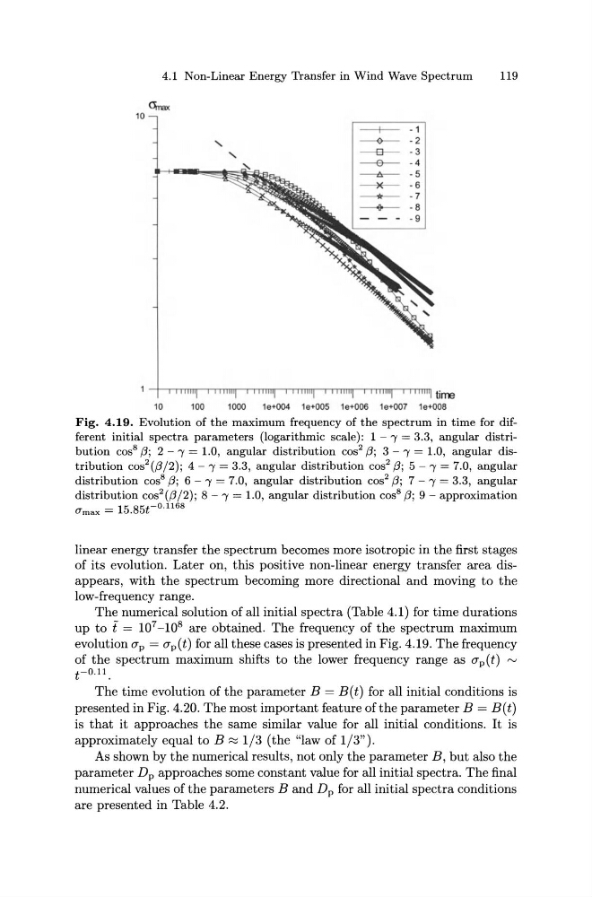
Fig. 4.19. Evolution of the maximum frequency of the spectrum in time for different initial spectra parameters (logarithmic scale): 1 - 'Y = 3.3, angular distribution cos 8 /3; 2 - 'Y = 1.0, angular distribution cos 2 /3; 3 - 'Y = 1.0, angular distribution cos 2 (/3/2); 4 - 'Y = 3.3, angular distribution cos 2 /3; 5 - 'Y = 7.0, angular
distribution cos 8 /3; 6 - 'Y = 7.0, angular distribution cos 2 /3; 7 - 'Y = 3.3, angular
distribution cos 2 (/3/2); 8 - 'Y = 1.0, angular distribution cos 8 /3; 9- approximation
O" max = 15.85t- 0 · 1168
linear energy transfer the spectrum becomes more isotropic in the first stages
of its evolution. Later on, this positive non-linear energy transfer area disappears, with the spectrum becoming more directional and moving to the
low-frequency range.
The numerical solution of all initial spectra (Table 4.1) for time durations
up to t = 10 7 - 10 8 are obtained. The frequency of the spectrum maximum
evolution ap = ap(t) for all these cases is presented in Fig. 4.19. The frequency
of the spectrum maximum shifts to the lower frequency range as ap(t) , . . . . . ,
t-0.11_
The time evolution of the parameter B = B(t) for all initial conditions is
presented in Fig. 4.20. The most important feature of the parameter B = B(t)
is that it approaches the same similar value for all initial conditions. It is
approximately equal to B:;::, 1/3 (the "law of 1/3" ).
As shown by the numerical results, not only the parameter B, but also the
parameter Dp approaches some constant value for all initial spectra. The final
numerical values of the parameters B and Dp for all initial spectra conditions
are presented in Table 4.2.
119
q,.,..
10
' '
--+-~
----6-~
---+-- 1
-2
-3
-4
- 5
- 6
- 7
-8
-9
time
10
100
1000
1e+004 1e+005 1e+006 1e+007 1e+008
Fig. 4.19. Evolution of the maximum frequency of the spectrum in time for different initial spectra parameters (logarithmic scale): 1 - 'Y = 3.3, angular distribution cos 8 /3; 2 - 'Y = 1.0, angular distribution cos 2 /3; 3 - 'Y = 1.0, angular distribution cos 2 (/3/2); 4 - 'Y = 3.3, angular distribution cos 2 /3; 5 - 'Y = 7.0, angular
distribution cos 8 /3; 6 - 'Y = 7.0, angular distribution cos 2 /3; 7 - 'Y = 3.3, angular
distribution cos 2 (/3/2); 8 - 'Y = 1.0, angular distribution cos 8 /3; 9- approximation
O" max = 15.85t- 0 · 1168
linear energy transfer the spectrum becomes more isotropic in the first stages
of its evolution. Later on, this positive non-linear energy transfer area disappears, with the spectrum becoming more directional and moving to the
low-frequency range.
The numerical solution of all initial spectra (Table 4.1) for time durations
up to t = 10 7 - 10 8 are obtained. The frequency of the spectrum maximum
evolution ap = ap(t) for all these cases is presented in Fig. 4.19. The frequency
of the spectrum maximum shifts to the lower frequency range as ap(t) , . . . . . ,
t-0.11_
The time evolution of the parameter B = B(t) for all initial conditions is
presented in Fig. 4.20. The most important feature of the parameter B = B(t)
is that it approaches the same similar value for all initial conditions. It is
approximately equal to B:;::, 1/3 (the "law of 1/3" ).
As shown by the numerical results, not only the parameter B, but also the
parameter Dp approaches some constant value for all initial spectra. The final
numerical values of the parameters B and Dp for all initial spectra conditions
are presented in Table 4.2.