

96
4 Physical Mechanisms Forming the Wave Spectrum in Deep Water
0.24219
0.24141
0.23906
-0.00010
-0.00039
-0.00156
-0.00625
-0.02500
-0 .1 0000
-0.30000
-0 .38750
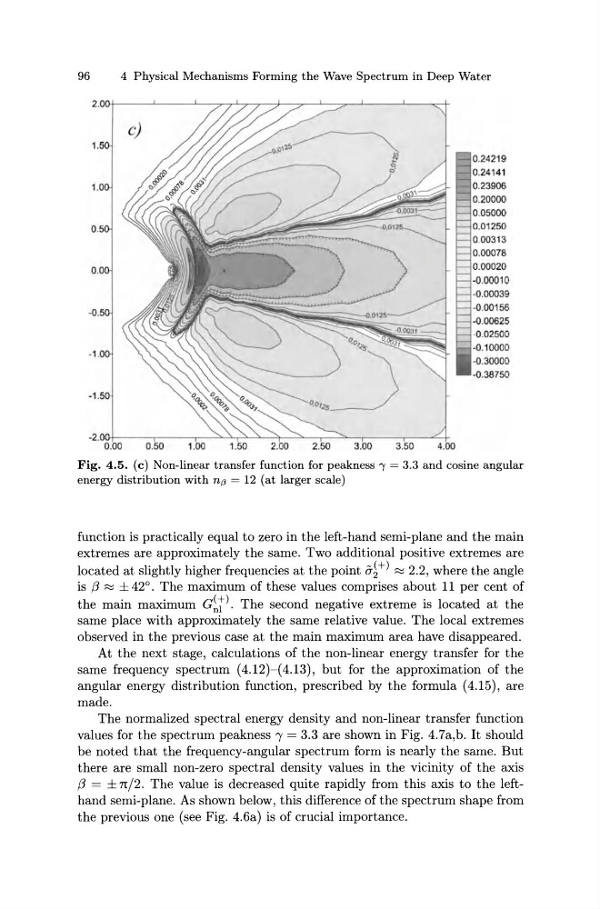
Fig. 4.5. (c) Non-linear transfer function for peakness 1 = 3.3 and cosine angular
energy distribution with n13 = 12 (at larger scale)
function is practically equal to zero in the left-hand semi-plane and the main
extremes are approximately the same. Two additional positive extremes are
located at slightly higher frequencies at the point a~+) ~ 2.2, where the angle
is f3 ~ ± 42°. The maximum of these values comprises about 11 per cent of
the main maximum G~i) . The second negative extreme is located at the
same place with approximately the same relative value. The local extremes
observed in the previous case at the main maximum area have disappeared.
At the next stage, calculations of the non-linear energy transfer for the
same frequency spectrum (4.12)- (4.13), but for the approximation of the
angular energy distribution function, prescribed by the formula (4.15), are
made.
The normalized spectral energy density and non-linear transfer function
values for the spectrum peakness I= 3.3 are shown in Fig. 4.7a,b. It should
be noted that the frequency-angular spectrum form is nearly the same. But
there are small non-zero spectral density values in the vicinity of the axis
f3 = ± n/2. The value is decreased quite rapidly from this axis to the lefthand semi-plane. As shown below, this difference of the spectrum shape from
the previous one (see Fig. 4.6a) is of crucial importance.
4 Physical Mechanisms Forming the Wave Spectrum in Deep Water
0.24219
0.24141
0.23906
-0.00010
-0.00039
-0.00156
-0.00625
-0.02500
-0 .1 0000
-0.30000
-0 .38750
Fig. 4.5. (c) Non-linear transfer function for peakness 1 = 3.3 and cosine angular
energy distribution with n13 = 12 (at larger scale)
function is practically equal to zero in the left-hand semi-plane and the main
extremes are approximately the same. Two additional positive extremes are
located at slightly higher frequencies at the point a~+) ~ 2.2, where the angle
is f3 ~ ± 42°. The maximum of these values comprises about 11 per cent of
the main maximum G~i) . The second negative extreme is located at the
same place with approximately the same relative value. The local extremes
observed in the previous case at the main maximum area have disappeared.
At the next stage, calculations of the non-linear energy transfer for the
same frequency spectrum (4.12)- (4.13), but for the approximation of the
angular energy distribution function, prescribed by the formula (4.15), are
made.
The normalized spectral energy density and non-linear transfer function
values for the spectrum peakness I= 3.3 are shown in Fig. 4.7a,b. It should
be noted that the frequency-angular spectrum form is nearly the same. But
there are small non-zero spectral density values in the vicinity of the axis
f3 = ± n/2. The value is decreased quite rapidly from this axis to the lefthand semi-plane. As shown below, this difference of the spectrum shape from
the previous one (see Fig. 4.6a) is of crucial importance.