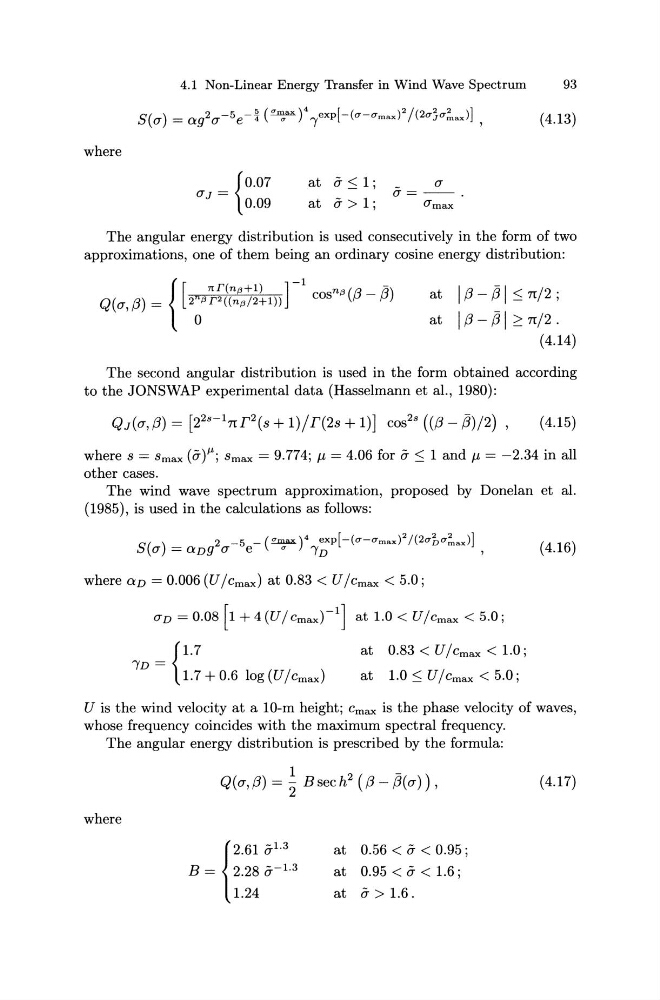
4.1 Non-Linear Energy Transfer in Wind Wave Spectrum
93
where
(J
= {0.07
J
0.09
at a :::: 1 ; -
(J
CY=--.
at a > 1 j
CYmax
The angular energy distribution is used consecutively in the form of two
approximations, one of them being an ordinary cosine energy distribution:
7t F(niJ+1)
nil
-
{
[
]
-1
Q(CY,{3) =
2;F2((ni3/2+1))
COS ({3- {3)
at I {3 - ;31 :=; nl2 ;
at I {3 - ;31 ?_ nl2 .
(4.14)
The second angular distribution is used in the form obtained according
to the JONSWAP experimental data (Hasselmann et al., 1980):
(4.15)
where S = Smax (a)"; Smax = 9.774; J1 = 4.06 for a :S: 1 and J1 = -2.34 in all
other cases.
The wind wave spectrum approximation, proposed by Donelan et al.
(1985), is used in the calculations as follows:
S( )
2 -5 - ( ==. t exp[-(a-O"max) 2 /(2ai,a~axl]
CY = avg CY e
"
TD
'
(4.16)
where av = 0.006 (U lcmax) at 0.83 < U lcmax < 5.0;
CYD = 0.08 [ 1 + 4 (U I Cmax)- 1 ] at 1.0 < U lcmax < 5.0;
{
1.7
/D =
1.7 + 0.6 log (Uicmax)
at 0.83 < u lcmax < 1.0;
at 1.0 :::: u I Crnax < 5.0;
U is the wind velocity at a 10-m height; Cmax is the phase velocity of waves,
whose frequency coincides with the maximum spectral frequency.
The angular energy distribution is prescribed by the formula:
where
Q(CY,{3) = ~ Bsech 2 (f3- ;3(CY)),
{
2.61 al.3
B = 2.28 a-1.3
1.24
at 0.56 at 0.95 < a < 1.6;
at a> 1.6.
(4.17)