

ANNE-MARIE TREGUIER
Evolution of a tracer by the diffusion equation
- 1
- - -
Initial ~rofile I
- Final profile I
-500;
0.2 I
0.4
0.6
0.8
Tracer
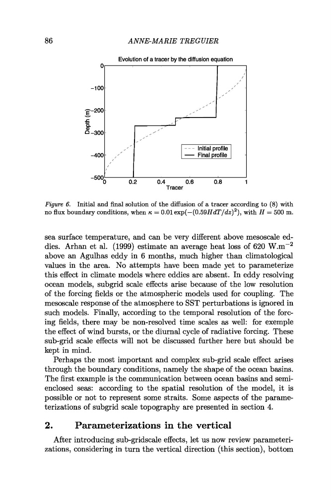
Figure 6. Initial and final solution of the diffusion of a tracer according to (8) with
no flux boundary conditions, when n = 0.01 e ~ ~ ( - ( 0 . 5 9 ~ d ~ / d z ) ~ ) ,
with H = 500 m.
sea surface temperature, and can be very different above mesoscale eddies. Arhan et al. (1999) estimate an average heat loss of 620 W.mP2
above an Agulhas eddy in 6 months, much higher than climatological
values in the area. No attempts have been made yet to parameterize
this effect in climate models where eddies are absent. In eddy resolving
ocean models, subgrid scale effects arise because of the low resolution
of the forcing fields or the atmospheric models used for coupling. The
mesoscale response of the atmosphere to SST perturbations is ignored in
such models. Finally, according to the temporal resolution of the forcing fields, there may be non-resolved time scales as well: for exemple
the effect of wind bursts, or the diurnal cycle of radiative forcing. These
sub-grid scale effects will not be discussed further here but should be
kept in mind.
Perhaps the most important and complex sub-grid scale effect arises
through the boundary conditions, namely the shape of the ocean basins.
The first example is the communication between ocean basins and semienclosed seas: according to the spatial resolution of the model, it is
possible or not to represent some straits. Some aspects of the parameterization~ of subgrid scale topography are presented in section 4.
2.
Parameterizations in the vertical
After introducing sub-gridscale effects, let us now review parameterization~, considering in turn the vertical direction (this section), bottom
Evolution of a tracer by the diffusion equation
- 1
- - -
Initial ~rofile I
- Final profile I
-500;
0.2 I
0.4
0.6
0.8
Tracer
Figure 6. Initial and final solution of the diffusion of a tracer according to (8) with
no flux boundary conditions, when n = 0.01 e ~ ~ ( - ( 0 . 5 9 ~ d ~ / d z ) ~ ) ,
with H = 500 m.
sea surface temperature, and can be very different above mesoscale eddies. Arhan et al. (1999) estimate an average heat loss of 620 W.mP2
above an Agulhas eddy in 6 months, much higher than climatological
values in the area. No attempts have been made yet to parameterize
this effect in climate models where eddies are absent. In eddy resolving
ocean models, subgrid scale effects arise because of the low resolution
of the forcing fields or the atmospheric models used for coupling. The
mesoscale response of the atmosphere to SST perturbations is ignored in
such models. Finally, according to the temporal resolution of the forcing fields, there may be non-resolved time scales as well: for exemple
the effect of wind bursts, or the diurnal cycle of radiative forcing. These
sub-grid scale effects will not be discussed further here but should be
kept in mind.
Perhaps the most important and complex sub-grid scale effect arises
through the boundary conditions, namely the shape of the ocean basins.
The first example is the communication between ocean basins and semienclosed seas: according to the spatial resolution of the model, it is
possible or not to represent some straits. Some aspects of the parameterization~ of subgrid scale topography are presented in section 4.
2.
Parameterizations in the vertical
After introducing sub-gridscale effects, let us now review parameterization~, considering in turn the vertical direction (this section), bottom