

OCEAN MODELS
79
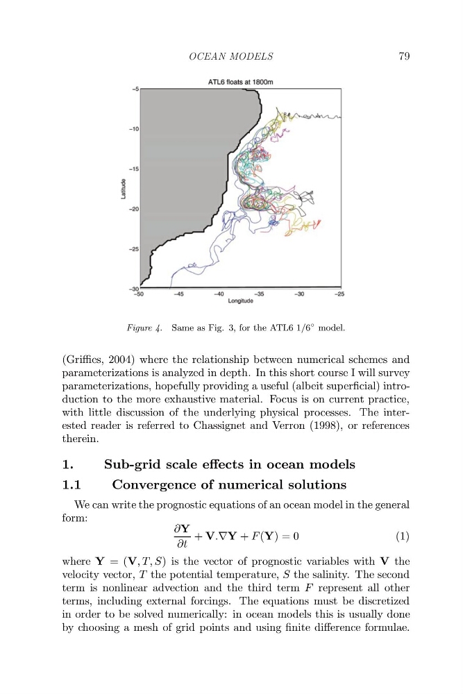
Figure 4. Same as Fig. 3, for the ATL6 1/6
◦ model.
(Griffies, 2004) where the relationship between numerical schemes and
parameterizations is analyzed in depth. In this short course I will survey
parameterizations, hopefully providing a useful (albeit superficial) introduction to the more exhaustive material. Focus is on current practice,
with little discussion of the underlying physical processes. The interested reader is referred to Chassignet and Verron (1998), or references
therein.
1.
Sub-grid scale effects in ocean models
1.1
Convergence of numerical solutions
We can write the prognostic equations of an ocean model in the general
form:
∂Y
∂t
+ V.∇Y + F (Y) = 0
(1)
where Y = (V, T, S) is the vector of prognostic variables with V the
velocity vector, T the potential temperature, S the salinity. The second
term is nonlinear advection and the third term F represent all other
terms, including external forcings. The equations must be discretized
in order to be solved numerically: in ocean models this is usually done
by choosing a mesh of grid points and using finite difference formulae.
79
Figure 4. Same as Fig. 3, for the ATL6 1/6
◦ model.
(Griffies, 2004) where the relationship between numerical schemes and
parameterizations is analyzed in depth. In this short course I will survey
parameterizations, hopefully providing a useful (albeit superficial) introduction to the more exhaustive material. Focus is on current practice,
with little discussion of the underlying physical processes. The interested reader is referred to Chassignet and Verron (1998), or references
therein.
1.
Sub-grid scale effects in ocean models
1.1
Convergence of numerical solutions
We can write the prognostic equations of an ocean model in the general
form:
∂Y
∂t
+ V.∇Y + F (Y) = 0
(1)
where Y = (V, T, S) is the vector of prognostic variables with V the
velocity vector, T the potential temperature, S the salinity. The second
term is nonlinear advection and the third term F represent all other
terms, including external forcings. The equations must be discretized
in order to be solved numerically: in ocean models this is usually done
by choosing a mesh of grid points and using finite difference formulae.