

DATA ASSIMILATION
337
increments of different partitions are summed together to correct the entire
model state and control (Eq 42). However, because of the approximations,
the resulting smoothed state and smoothed controls do not exactly satisfy the
model equations and are, strictly speaking, physically inconsistent. Instead,
estimates of a smoothed state that is fully consistent with the control are
derived by re-integrating the model in time using the smoothed control
estimates.
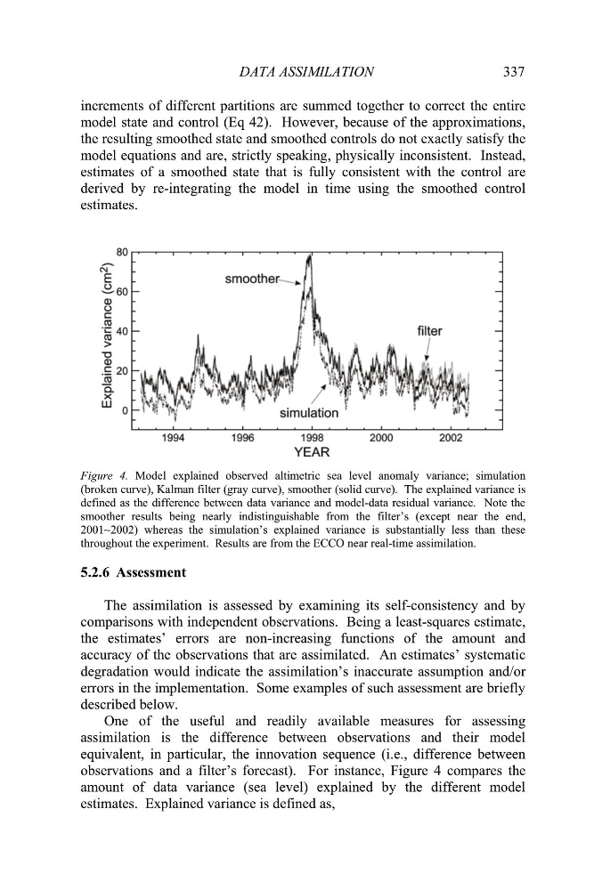
Figure 4. Model explained observed altimetric sea level anomaly variance; simulation
(broken curve), Kalman filter (gray curve), smoother (solid curve). The explained variance is
n is assessed by examining its self-consistency and by
omparisons with independent observations. Being a least-squares estimate,
the
e difference between observations and their model
equ
defined as the difference between data variance and model-data residual variance. Note the
smoother results being nearly indistinguishable from the filter’s (except near the end,
2001~2002) whereas the simulation’s explained variance is substantially less than these
throughout the experiment. Results are from the ECCO near real-time assimilation.
5.2.6 Assessment
The assimilatio
c
estimates’ errors are non-increasing functions of the amount and
accuracy of the observations that are assimilated. An estimates’ systematic
degradation would indicate the assimilation’s inaccurate assumption and/or
errors in the implementation. Some examples of such assessment are briefly
described below.
One of the useful and readily available measures for assessing
assimilation is th
ivalent, in particular, the innovation sequence (i.e., difference between
observations and a filter’s forecast). For instance, Figure 4 compares the
amount of data variance (sea level) explained by the different model
estimates. Explained variance is defined as,
337
increments of different partitions are summed together to correct the entire
model state and control (Eq 42). However, because of the approximations,
the resulting smoothed state and smoothed controls do not exactly satisfy the
model equations and are, strictly speaking, physically inconsistent. Instead,
estimates of a smoothed state that is fully consistent with the control are
derived by re-integrating the model in time using the smoothed control
estimates.
Figure 4. Model explained observed altimetric sea level anomaly variance; simulation
(broken curve), Kalman filter (gray curve), smoother (solid curve). The explained variance is
n is assessed by examining its self-consistency and by
omparisons with independent observations. Being a least-squares estimate,
the
e difference between observations and their model
equ
defined as the difference between data variance and model-data residual variance. Note the
smoother results being nearly indistinguishable from the filter’s (except near the end,
2001~2002) whereas the simulation’s explained variance is substantially less than these
throughout the experiment. Results are from the ECCO near real-time assimilation.
5.2.6 Assessment
The assimilatio
c
estimates’ errors are non-increasing functions of the amount and
accuracy of the observations that are assimilated. An estimates’ systematic
degradation would indicate the assimilation’s inaccurate assumption and/or
errors in the implementation. Some examples of such assessment are briefly
described below.
One of the useful and readily available measures for assessing
assimilation is th
ivalent, in particular, the innovation sequence (i.e., difference between
observations and a filter’s forecast). For instance, Figure 4 compares the
amount of data variance (sea level) explained by the different model
estimates. Explained variance is defined as,