

ICHIRO FUKUMORI
338
T
T
H
H
yy
y
x y
x
(44)
T
iance of what the model
cannot explai
variance (first term) is a
he second term, the residual variance, is the var
n, and thus the difference with the data
ulation without data
measure of what the model resolves. As the forecast does not yet utilize the
particular observations, the innovation sequence also provides a measure of
skill with respect to independent observations.
Figure 4 illustrates that the approximate Kalman filter explains
significantly more data variance than does the model sim
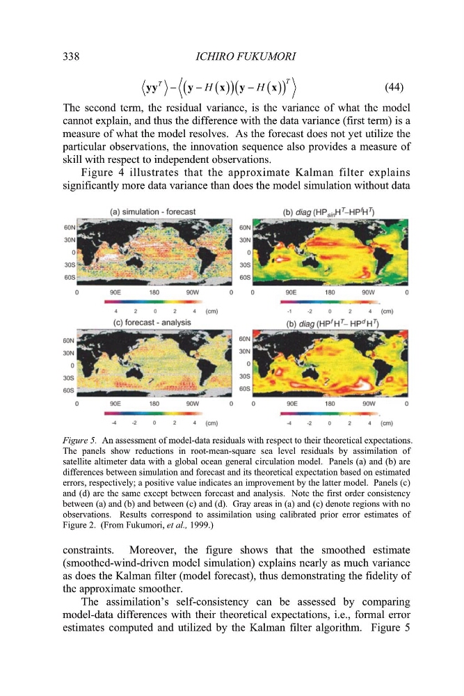
Figure 5. An assessment of model-data residuals with respect to their theoretical expectations.
The panels show reductions in root-mean-square sea level residuals by assimilation of
ure shows that the smoothed estimate
(sm thed-wind-driven model simulation) explains nearly as much variance
their theoretical expectations, i.e., formal error
estimates computed and utilized by the Kalman filter algorithm. Figure 5
satellite altimeter data with a global ocean general circulation model. Panels (a) and (b) are
differences between simulation and forecast and its theoretical expectation based on estimated
errors, respectively; a positive value indicates an improvement by the latter model. Panels (c)
and (d) are the same except between forecast and analysis. Note the first order consistency
between (a) and (b) and between (c) and (d). Gray areas in (a) and (c) denote regions with no
observations. Results correspond to assimilation using calibrated prior error estimates of
Figure 2. (From Fukumori, et al., 1999.)
constraints. Moreover, the fig
oo
as does the Kalman filter (model forecast), thus demonstrating the fidelity of
the approximate smoother.
The assimilation’s self-consistency can be assessed by comparing
model-data differences with
338
T
T
H
H
yy
y
x y
x
(44)
T
iance of what the model
cannot explai
variance (first term) is a
he second term, the residual variance, is the var
n, and thus the difference with the data
ulation without data
measure of what the model resolves. As the forecast does not yet utilize the
particular observations, the innovation sequence also provides a measure of
skill with respect to independent observations.
Figure 4 illustrates that the approximate Kalman filter explains
significantly more data variance than does the model sim
Figure 5. An assessment of model-data residuals with respect to their theoretical expectations.
The panels show reductions in root-mean-square sea level residuals by assimilation of
ure shows that the smoothed estimate
(sm thed-wind-driven model simulation) explains nearly as much variance
their theoretical expectations, i.e., formal error
estimates computed and utilized by the Kalman filter algorithm. Figure 5
satellite altimeter data with a global ocean general circulation model. Panels (a) and (b) are
differences between simulation and forecast and its theoretical expectation based on estimated
errors, respectively; a positive value indicates an improvement by the latter model. Panels (c)
and (d) are the same except between forecast and analysis. Note the first order consistency
between (a) and (b) and between (c) and (d). Gray areas in (a) and (c) denote regions with no
observations. Results correspond to assimilation using calibrated prior error estimates of
Figure 2. (From Fukumori, et al., 1999.)
constraints. Moreover, the fig
oo
as does the Kalman filter (model forecast), thus demonstrating the fidelity of
the approximate smoother.
The assimilation’s self-consistency can be assessed by comparing
model-data differences with