

DATA ASSIMILATION
333
ed reduced-state model and is
com
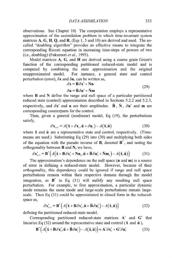
observations. See Chapter 10) The computation employs a representative
approximation of the assimilation problem in which time-invariant system
matrices A, G, H, Q, and R, (Eqs 1, 5 and 10) are derived and used. The socalled “doubling algorithm” provides an effective means to integrate the
corresponding Riccati equation in increasing time-steps of powers of two
(i.e., doubling) (Fukumori et al., 1993).
Model matrices A, G, and H are derived using a coarse grain Green's
function of the corresponding partition
puted by combining the state approximation and the original
unapproximated model.
For instance, a general state and control
perturbation (error), Gx and Gu, can be written as,
G
G
G
G
c
c
x = B x Nn
u = B u Nm
(29)
w
space of a particular partitioned
here B and N define the range and null
reduced state (control) approximation described in Sections 5.2.2 and 5.2.3,
respectively, and G c
x and n are their amplitudes. B
, N
, G c
u and m are
corresponding counterparts for the control.
Then, given a general (nonlinear) model, Eq ( 9)
satisfy,
1 , the perturbations
1
,
,
t
t
t
A
A
G
G
G
x = x
x u
u
x u
(30)
where x and are a representative state and control, respectively
eans e used.) Substituting Eq (29) into (30) and
u
. (Timem
multiplying both sides
ar
of the equation with the pseudo inverse of B, denoted
*
B , and noting the
orthogonality between B and N, we have,
*
1
,
t
t
t
t
t
A
A
G
G
G
c
c
c
x = B
x B x Nn u B u Nm
u
,
x
n and m
f error in defining a reduced-state model. However, beca
orth
(31)
The approximation’s dependence on the null space (
) is a source
o
use of their
ogonality, this dependency could be ignored if range and null space
perturbations remain within their respective domain through the model
integration, as
*
B in Eq (31) will nullify any resulting null space
perturbation. For example, to first approximation, a particular dynamic
mode remains the same mode and large-scale perturbations remain largescale. Then Eq (31) could be approximated in closed form in the reducedspace as,
*
1
,
,
t
t
t
A
A
G
G
G
c
c
c
x = B
x B x u B u
x u
(32)
defining the partitioned reduced-state model.
Corresponding partitioned reduced-state matrices
c
ǹ and
c
G that
linearize Eq (32) around the representative state and control ( and
x
u ),
*
,
,
t
t
t
t
A
A
G
G
G
G
c
c
c c
c
|
B
x B x u B u
x u
A x G uc
(33)
333
ed reduced-state model and is
com
observations. See Chapter 10) The computation employs a representative
approximation of the assimilation problem in which time-invariant system
matrices A, G, H, Q, and R, (Eqs 1, 5 and 10) are derived and used. The socalled “doubling algorithm” provides an effective means to integrate the
corresponding Riccati equation in increasing time-steps of powers of two
(i.e., doubling) (Fukumori et al., 1993).
Model matrices A, G, and H are derived using a coarse grain Green's
function of the corresponding partition
puted by combining the state approximation and the original
unapproximated model.
For instance, a general state and control
perturbation (error), Gx and Gu, can be written as,
G
G
G
G
c
c
x = B x Nn
u = B u Nm
(29)
w
space of a particular partitioned
here B and N define the range and null
reduced state (control) approximation described in Sections 5.2.2 and 5.2.3,
respectively, and G c
x and n are their amplitudes. B
, N
, G c
u and m are
corresponding counterparts for the control.
Then, given a general (nonlinear) model, Eq ( 9)
satisfy,
1 , the perturbations
1
,
,
t
t
t
A
A
G
G
G
x = x
x u
u
x u
(30)
where x and are a representative state and control, respectively
eans e used.) Substituting Eq (29) into (30) and
u
. (Timem
multiplying both sides
ar
of the equation with the pseudo inverse of B, denoted
*
B , and noting the
orthogonality between B and N, we have,
*
1
,
t
t
t
t
t
A
A
G
G
G
c
c
c
x = B
x B x Nn u B u Nm
u
,
x
n and m
f error in defining a reduced-state model. However, beca
orth
(31)
The approximation’s dependence on the null space (
) is a source
o
use of their
ogonality, this dependency could be ignored if range and null space
perturbations remain within their respective domain through the model
integration, as
*
B in Eq (31) will nullify any resulting null space
perturbation. For example, to first approximation, a particular dynamic
mode remains the same mode and large-scale perturbations remain largescale. Then Eq (31) could be approximated in closed form in the reducedspace as,
*
1
,
,
t
t
t
A
A
G
G
G
c
c
c
x = B
x B x u B u
x u
(32)
defining the partitioned reduced-state model.
Corresponding partitioned reduced-state matrices
c
ǹ and
c
G that
linearize Eq (32) around the representative state and control ( and
x
u ),
*
,
,
t
t
t
t
A
A
G
G
G
G
c
c
c c
c
|
B
x B x u B u
x u
A x G uc
(33)