

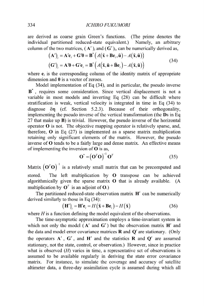
ICHIRO FUKUMORI
334
re derived as coarse grain Green’s functions. (The prim
equivalent.) Namely
a
e denotes the
individual partitioned reduced-state
, an arbitrary
column of the two matrices, ( c
ǹ ) i and ( c
G ) i , can be numerically derived as,
*
,
,
i
i
i
A
A
c
c
c
A
Ae G0 B
x Be u
x u
(34)
*
,
,
i
i
i
A
A
c
c
c
G
A0 Ge B
x u Be
x u
here e i is the corresponding column of the identity mat
dimension and 0 is a vector of zeroes.
vari
stra
w
rix of appropriate
Model implementation of Eq (34), and in particular, the pseudo inverse
*
B , requires some consideration. Since vertical displacement is not a
able in most models and inverting Eq (28) can be difficult where
tification is weak, vertical velocity is integrated in time in Eq (34) to
diagnose GK K (cf. Section 5.2.3). Because of their orthogonality,
implementing the pseudo inverse of the vertical transformation (the Ds in Eq
27 that make up B) is trivial. However, the pseudo inverse of the horizontal
operator O is not. The objective mapping operator is relatively sparse, and,
therefore, O in Eq (27) is implemented as a sparse matrix multiplication
retaining only significant elements of the matrix. However, the pseudo
inverse of O tends to be a fairly large and dense matrix. An effective means
of implementing the inversion of O is as,
1
*
T
T
O
O O O
(35)
Matrix
1
T
O O is a relatively small mat
mically
rix that can be precomputed and
stored.
The left multiplication by O transpose can be achieved
algorith
given the sparse matrix O that is already available. (A
multiplication by
T
O is an adjoint of O.)
The partitioned reduced-state observation matrix c
H can be numerically
derived similarly t hose in Eq (34):
o t
i
i
i
H
H
c
c
ning the model equivalent
The time-asymptotic approximation employs a
H
He
x Be
x
(36)
here H is a function defi
w
of the observations.
time-invariant system in
which not only the model ( c
ǹ and c
G ) but the observation matrix c
H and
the data and model error covariance matrices R and c
Q are stationary. (Only
the operators c
ǹ , c
G , and c
H and the statistics R and c
Q are assumed
stationary, not the state, control, or observation.) However, since in practice
what is observed (H varies i time, a representative set of observations is
assumed to be available regularly in deriving the state error covariance
matrix. For instance, to simulate the coverage and accuracy of satellite
altimeter data, a three-day assimilation cycle is assumed during which all
)
n
334
re derived as coarse grain Green’s functions. (The prim
equivalent.) Namely
a
e denotes the
individual partitioned reduced-state
, an arbitrary
column of the two matrices, ( c
ǹ ) i and ( c
G ) i , can be numerically derived as,
*
,
,
i
i
i
A
A
c
c
c
A
Ae G0 B
x Be u
x u
(34)
*
,
,
i
i
i
A
A
c
c
c
G
A0 Ge B
x u Be
x u
here e i is the corresponding column of the identity mat
dimension and 0 is a vector of zeroes.
vari
stra
w
rix of appropriate
Model implementation of Eq (34), and in particular, the pseudo inverse
*
B , requires some consideration. Since vertical displacement is not a
able in most models and inverting Eq (28) can be difficult where
tification is weak, vertical velocity is integrated in time in Eq (34) to
diagnose GK K (cf. Section 5.2.3). Because of their orthogonality,
implementing the pseudo inverse of the vertical transformation (the Ds in Eq
27 that make up B) is trivial. However, the pseudo inverse of the horizontal
operator O is not. The objective mapping operator is relatively sparse, and,
therefore, O in Eq (27) is implemented as a sparse matrix multiplication
retaining only significant elements of the matrix. However, the pseudo
inverse of O tends to be a fairly large and dense matrix. An effective means
of implementing the inversion of O is as,
1
*
T
T
O
O O O
(35)
Matrix
1
T
O O is a relatively small mat
mically
rix that can be precomputed and
stored.
The left multiplication by O transpose can be achieved
algorith
given the sparse matrix O that is already available. (A
multiplication by
T
O is an adjoint of O.)
The partitioned reduced-state observation matrix c
H can be numerically
derived similarly t hose in Eq (34):
o t
i
i
i
H
H
c
c
ning the model equivalent
The time-asymptotic approximation employs a
H
He
x Be
x
(36)
here H is a function defi
w
of the observations.
time-invariant system in
which not only the model ( c
ǹ and c
G ) but the observation matrix c
H and
the data and model error covariance matrices R and c
Q are stationary. (Only
the operators c
ǹ , c
G , and c
H and the statistics R and c
Q are assumed
stationary, not the state, control, or observation.) However, since in practice
what is observed (H varies i time, a representative set of observations is
assumed to be available regularly in deriving the state error covariance
matrix. For instance, to simulate the coverage and accuracy of satellite
altimeter data, a three-day assimilation cycle is assumed during which all
)
n