

ICHIRO FUKUMORI
322
¸
(8)
1
1
1
1
ˆ
ˆ
ˆ
ˆ
ˆ
s
a
s
s
t
t
t
t
s
t
§
·
¨
©
¹
x
x Ax
Gu
AG
u
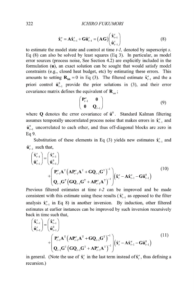
to estimate the model state and control at time t-1, denoted by superscript s.
Eq (8) can also be solved by least squares (Eq 3). In particular, as model
error sources (process noise, See Section 4.2) are explicitly included in the
formulation (u), an exact solution can be sought that would satisfy model
constraints (e.g., closed heat budget, etc) by estimating these errors. This
amounts to setting
in Eq (3). The filtered estimate
0
bb
R
1
ˆ
a
t
x and the a
priori control
provide the prior solutions in (3), and their error
covariance matrix defines the equivalent of
;
0
1
ˆ t
u
aa
R
(9)
1
1
a
t
t
§
·
¨
©
¹
P
0
0 Q
¸
where Q denotes the error covariance of
. Standard Kalman filtering
assumes temporally uncorrelated process noise that makes errors in
0
ˆ
u
1
ˆ
a
t
x and
0
1
ˆ t
u
Substitution of these elements in Eq (3) yields new estimates 1
ˆ
s
t
x and
1
ˆ
s
t
u such that,
(10)
1
1
0
1
1
1
T
T
T
1
1
1
0
1
1
1
T
T
T
1
1
1
ˆ
ˆ
ˆ
ˆ
ˆ
ˆ
ˆ
+
s
a
t
t
s
t
t
a
a
t
t
t
a
a
t
t
t
a
t
t
t
§
· §
·
¨
¸ ¨
¸
©
¹ ©
¹
§
·
¨
¸
¨
¸
¨
¸
©
¹
x
x
u
u
P A AP A GQ G
x Ax
Gu
Q G GQ G AP A
Previous filtered estimates at time t-2 can be improved and be made
consistent with this estimate using these results ( 1
ˆ
s
t
x as opposed to the filter
analysis
in Eq 8) in another inversion. By induction, other filtered
estimates at earlier instances can be improved by such inversion recursively
back in time such that,
1
ˆ
a
t
x
(11)
1
1
0
1
1
1
T
T
T
1
1
1
0
1
1
1
T
T
T
1
1
1
ˆ
ˆ
ˆ
ˆ
ˆ
ˆ
ˆ
+
s
a
t
t
s
t
t
a
a
t
t
t
s
a
t
t
t
a
t
t
t
§
· §
·
¨
¸ ¨
¸
©
¹ ©
¹
§
·
¨
¸
¨
¸
¨
¸
©
¹
x
x
u
u
P A AP A GQ G
x Ax
Gu
Q G GQ G AP A
in general. (Note the use of ˆ
s
t
x in the last term instead of , thus defining a
recursion.)
ˆ
a
t
x
uncorrelated to each other, and thus off-diagonal blocks are zero in
Eq 9.
322
¸
(8)
1
1
1
1
ˆ
ˆ
ˆ
ˆ
ˆ
s
a
s
s
t
t
t
t
s
t
§
·
¨
©
¹
x
x Ax
Gu
AG
u
to estimate the model state and control at time t-1, denoted by superscript s.
Eq (8) can also be solved by least squares (Eq 3). In particular, as model
error sources (process noise, See Section 4.2) are explicitly included in the
formulation (u), an exact solution can be sought that would satisfy model
constraints (e.g., closed heat budget, etc) by estimating these errors. This
amounts to setting
in Eq (3). The filtered estimate
0
bb
R
1
ˆ
a
t
x and the a
priori control
provide the prior solutions in (3), and their error
covariance matrix defines the equivalent of
;
0
1
ˆ t
u
aa
R
(9)
1
1
a
t
t
§
·
¨
©
¹
P
0
0 Q
¸
where Q denotes the error covariance of
. Standard Kalman filtering
assumes temporally uncorrelated process noise that makes errors in
0
ˆ
u
1
ˆ
a
t
x and
0
1
ˆ t
u
Substitution of these elements in Eq (3) yields new estimates 1
ˆ
s
t
x and
1
ˆ
s
t
u such that,
(10)
1
1
0
1
1
1
T
T
T
1
1
1
0
1
1
1
T
T
T
1
1
1
ˆ
ˆ
ˆ
ˆ
ˆ
ˆ
ˆ
+
s
a
t
t
s
t
t
a
a
t
t
t
a
a
t
t
t
a
t
t
t
§
· §
·
¨
¸ ¨
¸
©
¹ ©
¹
§
·
¨
¸
¨
¸
¨
¸
©
¹
x
x
u
u
P A AP A GQ G
x Ax
Gu
Q G GQ G AP A
Previous filtered estimates at time t-2 can be improved and be made
consistent with this estimate using these results ( 1
ˆ
s
t
x as opposed to the filter
analysis
in Eq 8) in another inversion. By induction, other filtered
estimates at earlier instances can be improved by such inversion recursively
back in time such that,
1
ˆ
a
t
x
(11)
1
1
0
1
1
1
T
T
T
1
1
1
0
1
1
1
T
T
T
1
1
1
ˆ
ˆ
ˆ
ˆ
ˆ
ˆ
ˆ
+
s
a
t
t
s
t
t
a
a
t
t
t
s
a
t
t
t
a
t
t
t
§
· §
·
¨
¸ ¨
¸
©
¹ ©
¹
§
·
¨
¸
¨
¸
¨
¸
©
¹
x
x
u
u
P A AP A GQ G
x Ax
Gu
Q G GQ G AP A
in general. (Note the use of ˆ
s
t
x in the last term instead of , thus defining a
recursion.)
ˆ
a
t
x
uncorrelated to each other, and thus off-diagonal blocks are zero in
Eq 9.