

DATA ASSIMILATION
321
evolution between
and
is physically inconsistent. For instance,
budgets of heat and other properties cannot be closed between the two
instances.
1
ˆ
a
t
x
ˆ
a
t
x
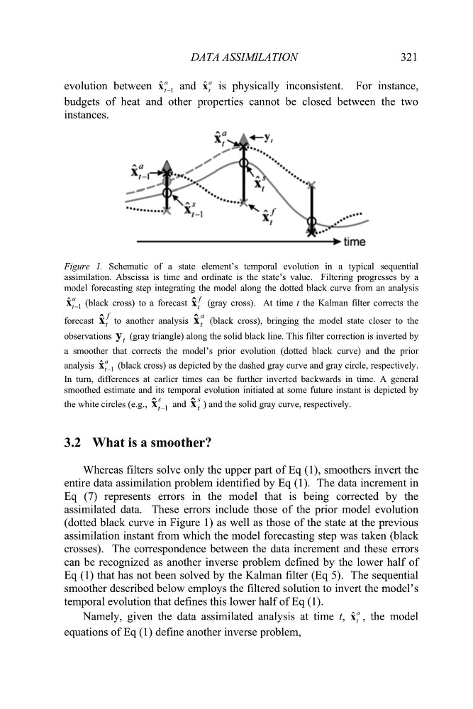
Figure 1. Schematic of a state element’s temporal evolution in a typical sequential
assimilation. Abscissa is time and ordinate is the state’s value. Filtering progresses by a
model forecasting step integrating the model along the dotted black curve from an analysis
(black cross) to a forecast
(gray cross). At time t the Kalman filter corrects the
forecast
to another analysis
(black cross), bringing the model state closer to the
observations
(gray triangle) along the solid black line. This filter correction is inverted by
a smoother that corrects the model’s prior evolution (dotted black curve) and the prior
analysis
(black cross) as depicted by the dashed gray curve and gray circle, respectively.
In turn, differences at earlier times can be further inverted backwards in time. A general
smoothed estimate and its temporal evolution initiated at some future instant is depicted by
the white circles (e.g.,
and
) and the solid gray curve, respectively.
1
ˆ
a
t
x
f
t
x ˆ
f
t
x ˆ
a
t
x ˆ
t
y
1
ˆ
a
t
x
s
t 1
x ˆ
s
t
x ˆ
3.2 What is a smoother?
Whereas filters solve only the upper part of Eq (1), smoothers invert the
entire data assimilation problem identified by Eq (1). The data increment in
Eq (7) represents errors in the model that is being corrected by the
assimilated data. These errors include those of the prior model evolution
(dotted black curve in Figure 1) as well as those of the state at the previous
assimilation instant from which the model forecasting step was taken (black
crosses). The correspondence between the data increment and these errors
can be recognized as another inverse problem defined by the lower half of
Eq (1) that has not been solved by the Kalman filter (Eq 5). The sequential
smoother described below employs the filtered solution to invert the model’s
temporal evolution that defines this lower half of Eq (1).
Namely, given the data assimilated analysis at time t,
, the model
equations of Eq (1) define another inverse problem,
ˆ
a
t
x
321
evolution between
and
is physically inconsistent. For instance,
budgets of heat and other properties cannot be closed between the two
instances.
1
ˆ
a
t
x
ˆ
a
t
x
Figure 1. Schematic of a state element’s temporal evolution in a typical sequential
assimilation. Abscissa is time and ordinate is the state’s value. Filtering progresses by a
model forecasting step integrating the model along the dotted black curve from an analysis
(black cross) to a forecast
(gray cross). At time t the Kalman filter corrects the
forecast
to another analysis
(black cross), bringing the model state closer to the
observations
(gray triangle) along the solid black line. This filter correction is inverted by
a smoother that corrects the model’s prior evolution (dotted black curve) and the prior
analysis
(black cross) as depicted by the dashed gray curve and gray circle, respectively.
In turn, differences at earlier times can be further inverted backwards in time. A general
smoothed estimate and its temporal evolution initiated at some future instant is depicted by
the white circles (e.g.,
and
) and the solid gray curve, respectively.
1
ˆ
a
t
x
f
t
x ˆ
f
t
x ˆ
a
t
x ˆ
t
y
1
ˆ
a
t
x
s
t 1
x ˆ
s
t
x ˆ
3.2 What is a smoother?
Whereas filters solve only the upper part of Eq (1), smoothers invert the
entire data assimilation problem identified by Eq (1). The data increment in
Eq (7) represents errors in the model that is being corrected by the
assimilated data. These errors include those of the prior model evolution
(dotted black curve in Figure 1) as well as those of the state at the previous
assimilation instant from which the model forecasting step was taken (black
crosses). The correspondence between the data increment and these errors
can be recognized as another inverse problem defined by the lower half of
Eq (1) that has not been solved by the Kalman filter (Eq 5). The sequential
smoother described below employs the filtered solution to invert the model’s
temporal evolution that defines this lower half of Eq (1).
Namely, given the data assimilated analysis at time t,
, the model
equations of Eq (1) define another inverse problem,
ˆ
a
t
x