

ICHIRO FUKUMORI
320
where
is a prior estimate of a, and
and
are prior error
covariance matrices of
and b, respectively. (The latter includes
representation error for E. See Section 4.1 for further discussion.) Filtering
and smoothing algorithms can be identified as such least squares inversions
and are reviewed below focusing on what they respectively solve.
0
a
aa
R
bb
R
0
a
A least-squares solution is identical to a minimum variance estimate
when weights used in least-squares are suitable inverse error covariance
matrices. These solutions are optimal in the sense that they optimize a given
criteria (function) and that the expected error variance of is minimum
among all (linear) estimates. Least-squares, as well as filtering and
smoothing described below, do not necessarily assume Gaussian statistics.
When the statistical distribution of a is Gaussian, the least-squares estimate
is also a maximum likelihood estimate. Otherwise, the least-squares solution
and the maximum likelihood estimate are distinct.
ˆ
a
3.1 What do Kalman filters solve?
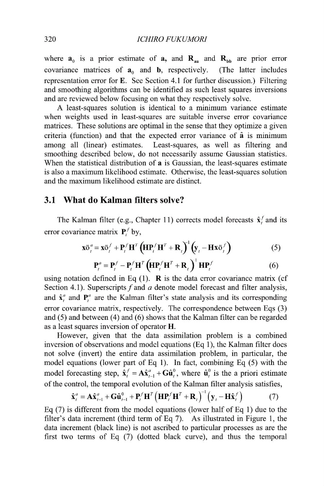
The Kalman filter (e.g., Chapter 11) corrects model forecasts ˆ
f
t
x and its
error covariance matrix
f
t
P by,
ö
x t
a
ö
x t
f P t
f H
T HP t
f H
T R t
1
y t H ö
x t
f
(5)
(6)
P t
a
P t
f P t
f H
T HP t
f H
T R t
1
HP t
f
using notation defined in Eq (1). R is the data error covariance matrix (cf
Section 4.1). Superscripts f and a denote model forecast and filter analysis,
and
and
are the Kalman filter’s state analysis and its corresponding
error covariance matrix, respectively. The correspondence between Eqs (3)
and (5) and between (4) and (6) shows that the Kalman filter can be regarded
as a least squares inversion of operator H.
ˆ
a
t
x
a
t
P
However, given that the data assimilation problem is a combined
inversion of observations and model equations (Eq 1), the Kalman filter does
not solve (invert) the entire data assimilation problem, in particular, the
model equations (lower part of Eq 1). In fact, combining Eq (5) with the
model forecasting step,
, where
is the a priori estimate
of the control, the temporal evolution of the Kalman filter analysis satisfies,
0
1
ˆ
ˆ
f
a
t
t
x
Ax
Gu ˆ t
0
ˆ t
u
1
0
1
1
ˆ
ˆ
ˆ
ˆ
a
a
f
T
f
T
f
t
t
t
t
t
t
t
t
x Ax
Gu
P H HP H R
y Hx
(7)
Eq (7) is different from the model equations (lower half of Eq 1) due to the
filter’s data increment (third term of Eq 7). As illustrated in Figure 1, the
data increment (black line) is not ascribed to particular processes as are the
first two terms of Eq (7) (dotted black curve), and thus the temporal
320
where
is a prior estimate of a, and
and
are prior error
covariance matrices of
and b, respectively. (The latter includes
representation error for E. See Section 4.1 for further discussion.) Filtering
and smoothing algorithms can be identified as such least squares inversions
and are reviewed below focusing on what they respectively solve.
0
a
aa
R
bb
R
0
a
A least-squares solution is identical to a minimum variance estimate
when weights used in least-squares are suitable inverse error covariance
matrices. These solutions are optimal in the sense that they optimize a given
criteria (function) and that the expected error variance of is minimum
among all (linear) estimates. Least-squares, as well as filtering and
smoothing described below, do not necessarily assume Gaussian statistics.
When the statistical distribution of a is Gaussian, the least-squares estimate
is also a maximum likelihood estimate. Otherwise, the least-squares solution
and the maximum likelihood estimate are distinct.
ˆ
a
3.1 What do Kalman filters solve?
The Kalman filter (e.g., Chapter 11) corrects model forecasts ˆ
f
t
x and its
error covariance matrix
f
t
P by,
ö
x t
a
ö
x t
f P t
f H
T HP t
f H
T R t
1
y t H ö
x t
f
(5)
(6)
P t
a
P t
f P t
f H
T HP t
f H
T R t
1
HP t
f
using notation defined in Eq (1). R is the data error covariance matrix (cf
Section 4.1). Superscripts f and a denote model forecast and filter analysis,
and
and
are the Kalman filter’s state analysis and its corresponding
error covariance matrix, respectively. The correspondence between Eqs (3)
and (5) and between (4) and (6) shows that the Kalman filter can be regarded
as a least squares inversion of operator H.
ˆ
a
t
x
a
t
P
However, given that the data assimilation problem is a combined
inversion of observations and model equations (Eq 1), the Kalman filter does
not solve (invert) the entire data assimilation problem, in particular, the
model equations (lower part of Eq 1). In fact, combining Eq (5) with the
model forecasting step,
, where
is the a priori estimate
of the control, the temporal evolution of the Kalman filter analysis satisfies,
0
1
ˆ
ˆ
f
a
t
t
x
Ax
Gu ˆ t
0
ˆ t
u
1
0
1
1
ˆ
ˆ
ˆ
ˆ
a
a
f
T
f
T
f
t
t
t
t
t
t
t
t
x Ax
Gu
P H HP H R
y Hx
(7)
Eq (7) is different from the model equations (lower half of Eq 1) due to the
filter’s data increment (third term of Eq 7). As illustrated in Figure 1, the
data increment (black line) is not ascribed to particular processes as are the
first two terms of Eq (7) (dotted black curve), and thus the temporal