

297
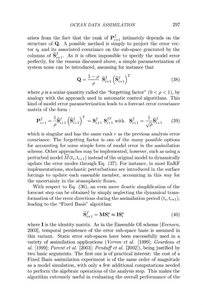
arises from the fact that the rank of P
f
i+1 intimately depends on the
structure of Q. A possible method is simply to project the error vector i and its associated covariance on the sub-space generated by the
columns of h
S
f
i+1 . As it is often impossible to specify the model error
perfectly, for the reasons discussed above, a simple parameterization of
system noise can be introduced, assuming for instance that
Q =
1
h
S
f
i+1
h
S
f
i+1
T
(38)
where is a scalar quantity called the “forgetting factor” (0 < < 1), by
analogy with the approach used in automatic control algorithms. This
kind of model error parameterization leads to a forecast error covariance
matrix of the form :
P
f
i+1 =
1
h
S
f
i+1
h
S
f
i+1
T = S
f
i+1 S
fT
i+1 with S
f
i+1 =
1
s
h
S
f
i+1
(39)
which is singular and has the same rank r as the previous analysis error
covariance. The forgetting factor is one of the many possible options
for accounting for some simple form of model error in the assimilation
scheme. Other approaches may be implemented, however, such as using a
perturbed model i
M (t i , t i+1 ) instead of the original model to dynamically
update the error modes through Eq. (37). For instance, in most EnKF
implementations, stochastic perturbations are introduced in the surface
forcings to update each ensemble member, accounting in this way for
the uncertainty in the atmospheric fluxes.
With respect to Eq. (36), an even more drastic simplification of the
forecast step can be obtained by simply neglecting the dynamical transformation of the error directions during the assimilation period (t i , t i+1 ),
leading to the “Fixed Basis” algorithm:
h
S
f
i+1 = MS
a
i r IS
a
i
(40)
where I is the identity matrix. As in the Ensemble OI scheme [Evensen,
2003], temporal persistence of the error sub-space basis is assumed in
this variant. Static error sub-spaces have been successfully used in a
variety of assimilation applications (Verron et al. [1999]; Gourdeau et
al. [1999]; Parent et al. [2003]; Pendu et al. [2002]), being justified by
two basic arguments. The first one is of practical interest: the cost of a
Fixed Basis assimilation experiment is of the same order of magnitude
as a model simulation, with only a few additional computations needed
to perform the algebraic operations of the analysis step. This makes the
algorithm extremely useful in evaluating the overall performance of the
OCEAN DATA ASSIMILATION
arises from the fact that the rank of P
f
i+1 intimately depends on the
structure of Q. A possible method is simply to project the error vector i and its associated covariance on the sub-space generated by the
columns of h
S
f
i+1 . As it is often impossible to specify the model error
perfectly, for the reasons discussed above, a simple parameterization of
system noise can be introduced, assuming for instance that
Q =
1
h
S
f
i+1
h
S
f
i+1
T
(38)
where is a scalar quantity called the “forgetting factor” (0 < < 1), by
analogy with the approach used in automatic control algorithms. This
kind of model error parameterization leads to a forecast error covariance
matrix of the form :
P
f
i+1 =
1
h
S
f
i+1
h
S
f
i+1
T = S
f
i+1 S
fT
i+1 with S
f
i+1 =
1
s
h
S
f
i+1
(39)
which is singular and has the same rank r as the previous analysis error
covariance. The forgetting factor is one of the many possible options
for accounting for some simple form of model error in the assimilation
scheme. Other approaches may be implemented, however, such as using a
perturbed model i
M (t i , t i+1 ) instead of the original model to dynamically
update the error modes through Eq. (37). For instance, in most EnKF
implementations, stochastic perturbations are introduced in the surface
forcings to update each ensemble member, accounting in this way for
the uncertainty in the atmospheric fluxes.
With respect to Eq. (36), an even more drastic simplification of the
forecast step can be obtained by simply neglecting the dynamical transformation of the error directions during the assimilation period (t i , t i+1 ),
leading to the “Fixed Basis” algorithm:
h
S
f
i+1 = MS
a
i r IS
a
i
(40)
where I is the identity matrix. As in the Ensemble OI scheme [Evensen,
2003], temporal persistence of the error sub-space basis is assumed in
this variant. Static error sub-spaces have been successfully used in a
variety of assimilation applications (Verron et al. [1999]; Gourdeau et
al. [1999]; Parent et al. [2003]; Pendu et al. [2002]), being justified by
two basic arguments. The first one is of practical interest: the cost of a
Fixed Basis assimilation experiment is of the same order of magnitude
as a model simulation, with only a few additional computations needed
to perform the algebraic operations of the analysis step. This makes the
algorithm extremely useful in evaluating the overall performance of the
OCEAN DATA ASSIMILATION