

296
PIERRE BRASSEUR
6.1
Forecast error with a reduced basis
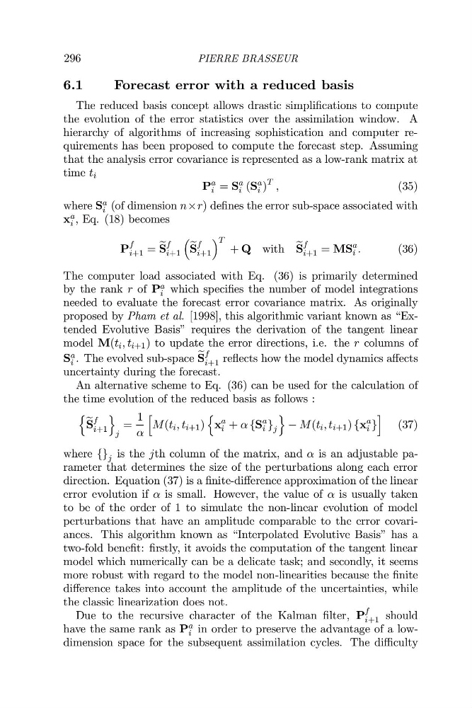
The reduced basis concept allows drastic simplifications to compute
the evolution of the error statistics over the assimilation window. A
hierarchy of algorithms of increasing sophistication and computer requirements has been proposed to compute the forecast step. Assuming
that the analysis error covariance is represented as a low-rank matrix at
time t i
P
a
i = S
a
i (S
a
i )
T ,
(35)
where S a
i (of dimension n×r) defines the error sub-space associated with
x a
i , Eq. (18) becomes
P
f
i+1 = h
S
f
i+1
h
S
f
i+1
T + Q with h
S
f
i+1 = MS
a
i .
(36)
The computer load associated with Eq. (36) is primarily determined
by the rank r of P a
i which specifies the number of model integrations
needed to evaluate the forecast error covariance matrix. As originally
proposed by Pham et al. [1998], this algorithmic variant known as “Extended Evolutive Basis” requires the derivation of the tangent linear
model M(t i , t i+1 ) to update the error directions, i.e. the r columns of
S a
i . The evolved sub-space h
S
f
i+1 reflects how the model dynamics aects
uncertainty during the forecast.
An alternative scheme to Eq. (36) can be used for the calculation of
the time evolution of the reduced basis as follows :
q
h
S
f
i+1
r
j
=
1
k
M(t i , t i+1 )
q
x
a
i + {S
a
i } j
r
M(t i , t i+1 ) {x
a
i }
l
(37)
where {} j is the jth column of the matrix, and is an adjustable parameter that determines the size of the perturbations along each error
direction. Equation (37) is a finite-dierence approximation of the linear
error evolution if is small. However, the value of is usually taken
to be of the order of 1 to simulate the non-linear evolution of model
perturbations that have an amplitude comparable to the error covariances. This algorithm known as “Interpolated Evolutive Basis” has a
two-fold benefit: firstly, it avoids the computation of the tangent linear
model which numerically can be a delicate task; and secondly, it seems
more robust with regard to the model non-linearities because the finite
dierence takes into account the amplitude of the uncertainties, while
the classic linearization does not.
Due to the recursive character of the Kalman filter, P
f
i+1 should
have the same rank as P
a
i in order to preserve the advantage of a lowdimension space for the subsequent assimilation cycles. The di!culty
PIERRE BRASSEUR
6.1
Forecast error with a reduced basis
The reduced basis concept allows drastic simplifications to compute
the evolution of the error statistics over the assimilation window. A
hierarchy of algorithms of increasing sophistication and computer requirements has been proposed to compute the forecast step. Assuming
that the analysis error covariance is represented as a low-rank matrix at
time t i
P
a
i = S
a
i (S
a
i )
T ,
(35)
where S a
i (of dimension n×r) defines the error sub-space associated with
x a
i , Eq. (18) becomes
P
f
i+1 = h
S
f
i+1
h
S
f
i+1
T + Q with h
S
f
i+1 = MS
a
i .
(36)
The computer load associated with Eq. (36) is primarily determined
by the rank r of P a
i which specifies the number of model integrations
needed to evaluate the forecast error covariance matrix. As originally
proposed by Pham et al. [1998], this algorithmic variant known as “Extended Evolutive Basis” requires the derivation of the tangent linear
model M(t i , t i+1 ) to update the error directions, i.e. the r columns of
S a
i . The evolved sub-space h
S
f
i+1 reflects how the model dynamics aects
uncertainty during the forecast.
An alternative scheme to Eq. (36) can be used for the calculation of
the time evolution of the reduced basis as follows :
q
h
S
f
i+1
r
j
=
1
k
M(t i , t i+1 )
q
x
a
i + {S
a
i } j
r
M(t i , t i+1 ) {x
a
i }
l
(37)
where {} j is the jth column of the matrix, and is an adjustable parameter that determines the size of the perturbations along each error
direction. Equation (37) is a finite-dierence approximation of the linear
error evolution if is small. However, the value of is usually taken
to be of the order of 1 to simulate the non-linear evolution of model
perturbations that have an amplitude comparable to the error covariances. This algorithm known as “Interpolated Evolutive Basis” has a
two-fold benefit: firstly, it avoids the computation of the tangent linear
model which numerically can be a delicate task; and secondly, it seems
more robust with regard to the model non-linearities because the finite
dierence takes into account the amplitude of the uncertainties, while
the classic linearization does not.
Due to the recursive character of the Kalman filter, P
f
i+1 should
have the same rank as P
a
i in order to preserve the advantage of a lowdimension space for the subsequent assimilation cycles. The di!culty