

298
PIERRE BRASSEUR
system, testing new parameterizations, examining the impact of dierent observation configurations, etc. The second argument constitutes a
more objective justification in terms of statistical estimation: it is often
impossible to properly characterize the statistical structure of the model
error originating from imperfections in the model forcings, discretization schemes, space/time resolution, etc. As a result, the approximation
made by assuming persistence of the error sub-space directions is often
negligible compared to the mis-specification of the systematic errors.
When the amplitude of the model error increment Q dominates the difference between P a and MP a M T in the error propagation Eq. (18), it
is a waste of CPU resources to explicitly compute the error propagation
with the model dynamics, because the result will eventually be polluted
by mis-specified model error estimates. In such situations, it is sensible
to by-pass the error propagation equation and concentrate on identifying the dominant forecast error directions using, for instance, adaptivity
mechanisms as described in Section 7.
6.2
Analysis step with a reduced basis
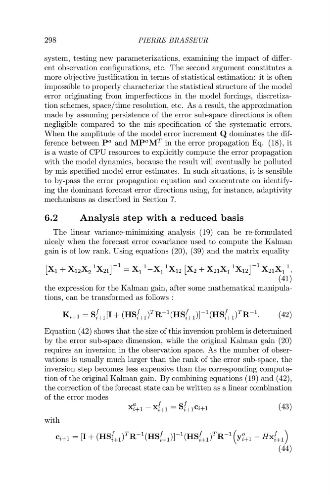
The linear variance-minimizing analysis (19) can be re-formulated
nicely when the forecast error covariance used to compute the Kalman
gain is of low rank. Using equations (20), (39) and the matrix equality
X 1 + X 12 X
31
2 X 21
31 = X
31
1 X
31
1 X 12
X 2 + X 21 X
31
1 X 12
31 X 21 X
31
1 ,
(41)
the expression for the Kalman gain, after some mathematical manipulations, can be transformed as follows :
K i+1 = S
f
i+1 [I + (HS
f
i+1 )
T R
31
(HS
f
i+1 )]
31
(HS
f
i+1 )
T R
31 .
(42)
Equation (42) shows that the size of this inversion problem is determined
by the error sub-space dimension, while the original Kalman gain (20)
requires an inversion in the observation space. As the number of observations is usually much larger than the rank of the error sub-space, the
inversion step becomes less expensive than the corresponding computation of the original Kalman gain. By combining equations (19) and (42),
the correction of the forecast state can be written as a linear combination
of the error modes
x
a
i+1 x
f
i+1 = S
f
i+1 c i+1
(43)
with
c i+1 = [I + (HS
f
i+1 )
T R
31
(HS
f
i+1 )]
31
(HS
f
i+1 )
T R
31
y
o
i+1 Hx
f
i+1
(44)
PIERRE BRASSEUR
system, testing new parameterizations, examining the impact of dierent observation configurations, etc. The second argument constitutes a
more objective justification in terms of statistical estimation: it is often
impossible to properly characterize the statistical structure of the model
error originating from imperfections in the model forcings, discretization schemes, space/time resolution, etc. As a result, the approximation
made by assuming persistence of the error sub-space directions is often
negligible compared to the mis-specification of the systematic errors.
When the amplitude of the model error increment Q dominates the difference between P a and MP a M T in the error propagation Eq. (18), it
is a waste of CPU resources to explicitly compute the error propagation
with the model dynamics, because the result will eventually be polluted
by mis-specified model error estimates. In such situations, it is sensible
to by-pass the error propagation equation and concentrate on identifying the dominant forecast error directions using, for instance, adaptivity
mechanisms as described in Section 7.
6.2
Analysis step with a reduced basis
The linear variance-minimizing analysis (19) can be re-formulated
nicely when the forecast error covariance used to compute the Kalman
gain is of low rank. Using equations (20), (39) and the matrix equality
X 1 + X 12 X
31
2 X 21
31 = X
31
1 X
31
1 X 12
X 2 + X 21 X
31
1 X 12
31 X 21 X
31
1 ,
(41)
the expression for the Kalman gain, after some mathematical manipulations, can be transformed as follows :
K i+1 = S
f
i+1 [I + (HS
f
i+1 )
T R
31
(HS
f
i+1 )]
31
(HS
f
i+1 )
T R
31 .
(42)
Equation (42) shows that the size of this inversion problem is determined
by the error sub-space dimension, while the original Kalman gain (20)
requires an inversion in the observation space. As the number of observations is usually much larger than the rank of the error sub-space, the
inversion step becomes less expensive than the corresponding computation of the original Kalman gain. By combining equations (19) and (42),
the correction of the forecast state can be written as a linear combination
of the error modes
x
a
i+1 x
f
i+1 = S
f
i+1 c i+1
(43)
with
c i+1 = [I + (HS
f
i+1 )
T R
31
(HS
f
i+1 )]
31
(HS
f
i+1 )
T R
31
y
o
i+1 Hx
f
i+1
(44)