

278
PIERRE BRASSEUR
and the optimal estimate becomes a perfect fit of the observations. By
contrast, if the forecast is extremely accurate (P
f 0) compared with
the observations, the correction is negligible. Interesting similarities between this equation and scalar formulations of least squares problems
can be found in Kalnay [2003]. Equation (15) is the second fundamental equation of the Kalman filter.
2.4
The sequential assimilation cycle
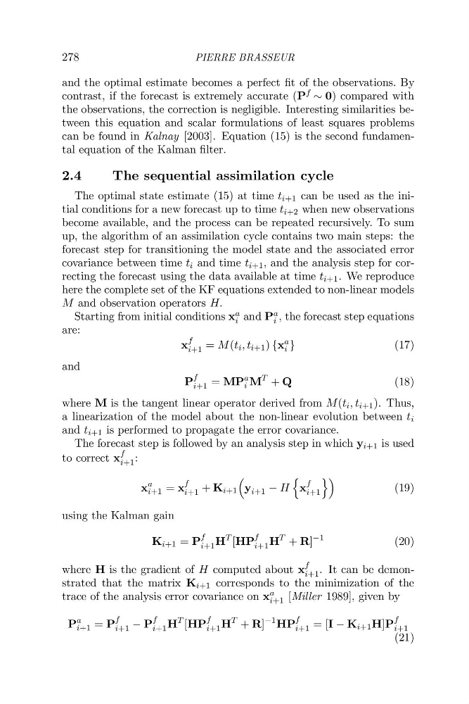
The optimal state estimate (15) at time t i+1 can be used as the initial conditions for a new forecast up to time t i+2 when new observations
become available, and the process can be repeated recursively. To sum
up, the algorithm of an assimilation cycle contains two main steps: the
forecast step for transitioning the model state and the associated error
covariance between time t i and time t i+1 , and the analysis step for correcting the forecast using the data available at time t i+1 . We reproduce
here the complete set of the KF equations extended to non-linear models
M and observation operators H.
Starting from initial conditions x a
i and P a
i , the forecast step equations
are:
x
f
i+1 = M(t i , t i+1 ) {x
a
i }
(17)
and
P
f
i+1 = MP
a
i M
T
+ Q
(18)
where M is the tangent linear operator derived from M(t i , t i+1 ). Thus,
a linearization of the model about the non-linear evolution between t i
and t i+1 is performed to propagate the error covariance.
The forecast step is followed by an analysis step in which y i+1 is used
to correct x
f
i+1 :
x
a
i+1 = x
f
i+1 + K i+1
y i+1 H
q
x
f
i+1
r
(19)
using the Kalman gain
K i+1 = P
f
i+1 H
T
[HP
f
i+1 H
T
+ R]
31
(20)
where H is the gradient of H computed about x
f
i+1 . It can be demonstrated that the matrix K i+1 corresponds to the minimization of the
trace of the analysis error covariance on x
a
i+1 [Miller 1989], given by
P
a
i+1 = P
f
i+1 P
f
i+1 H
T
[HP
f
i+1 H
T
+ R]
31 HP
f
i+1 = [I K i+1 H]P
f
i+1
(21)
PIERRE BRASSEUR
and the optimal estimate becomes a perfect fit of the observations. By
contrast, if the forecast is extremely accurate (P
f 0) compared with
the observations, the correction is negligible. Interesting similarities between this equation and scalar formulations of least squares problems
can be found in Kalnay [2003]. Equation (15) is the second fundamental equation of the Kalman filter.
2.4
The sequential assimilation cycle
The optimal state estimate (15) at time t i+1 can be used as the initial conditions for a new forecast up to time t i+2 when new observations
become available, and the process can be repeated recursively. To sum
up, the algorithm of an assimilation cycle contains two main steps: the
forecast step for transitioning the model state and the associated error
covariance between time t i and time t i+1 , and the analysis step for correcting the forecast using the data available at time t i+1 . We reproduce
here the complete set of the KF equations extended to non-linear models
M and observation operators H.
Starting from initial conditions x a
i and P a
i , the forecast step equations
are:
x
f
i+1 = M(t i , t i+1 ) {x
a
i }
(17)
and
P
f
i+1 = MP
a
i M
T
+ Q
(18)
where M is the tangent linear operator derived from M(t i , t i+1 ). Thus,
a linearization of the model about the non-linear evolution between t i
and t i+1 is performed to propagate the error covariance.
The forecast step is followed by an analysis step in which y i+1 is used
to correct x
f
i+1 :
x
a
i+1 = x
f
i+1 + K i+1
y i+1 H
q
x
f
i+1
r
(19)
using the Kalman gain
K i+1 = P
f
i+1 H
T
[HP
f
i+1 H
T
+ R]
31
(20)
where H is the gradient of H computed about x
f
i+1 . It can be demonstrated that the matrix K i+1 corresponds to the minimization of the
trace of the analysis error covariance on x
a
i+1 [Miller 1989], given by
P
a
i+1 = P
f
i+1 P
f
i+1 H
T
[HP
f
i+1 H
T
+ R]
31 HP
f
i+1 = [I K i+1 H]P
f
i+1
(21)