

120
RAINER BLECK
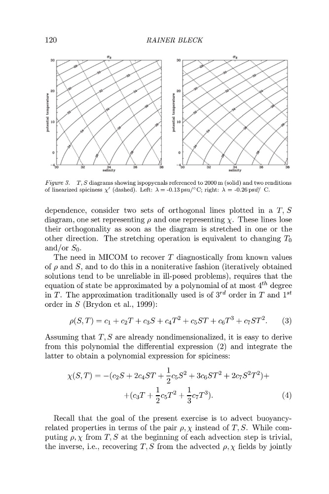
Figure 3. T, S diagrams showing ispopycnals referenced to 2000 m (solid) and two renditions
of linearized spiciness χ (dashed). Left: λ = -0.13 psu/ ◦ C; right: λ = -0.26 psu/ ◦ C.
dependence, consider two sets of orthogonal lines plotted in a T, S
diagram, one set representing ρ and one representing χ. These lines lose
their orthogonality as soon as the diagram is stretched in one or the
other direction. The stretching operation is equivalent to changing T 0
and/or S 0 .
The need in MICOM to recover T diagnostically from known values
of ρ and S, and to do this in a noniterative fashion (iteratively obtained
solutions tend to be unreliable in ill-posed problems), requires that the
equation of state be approximated by a polynomial of at most 4 th degree
in T . The approximation traditionally used is of 3 rd order in T and 1 st
order in S (Brydon et al., 1999):
ρ(S, T ) = c 1 + c 2 T + c 3 S + c 4 T
2 + c 5 ST + c 6 T
3 + c 7 ST
2 .
(3)
Assuming that T, S are already nondimensionalized, it is easy to derive
from this polynomial the differential expression (2) and integrate the
latter to obtain a polynomial expression for spiciness:
χ(S, T ) = −(c 2 S + 2c 4 ST +
1
2
c 5 S
2 + 3c 6 ST
2 + 2c 7 S
2 T
2 )+
+(c 3 T +
1
2
c 5 T
2 +
1
3
c 7 T
3 ).
(4)
Recall that the goal of the present exercise is to advect buoyancyrelated properties in terms of the pair ρ, χ instead of T, S. While computing ρ, χ from T, S at the beginning of each advection step is trivial,
the inverse, i.e., recovering T, S from the advected ρ, χ fields by jointly
RAINER BLECK
Figure 3. T, S diagrams showing ispopycnals referenced to 2000 m (solid) and two renditions
of linearized spiciness χ (dashed). Left: λ = -0.13 psu/ ◦ C; right: λ = -0.26 psu/ ◦ C.
dependence, consider two sets of orthogonal lines plotted in a T, S
diagram, one set representing ρ and one representing χ. These lines lose
their orthogonality as soon as the diagram is stretched in one or the
other direction. The stretching operation is equivalent to changing T 0
and/or S 0 .
The need in MICOM to recover T diagnostically from known values
of ρ and S, and to do this in a noniterative fashion (iteratively obtained
solutions tend to be unreliable in ill-posed problems), requires that the
equation of state be approximated by a polynomial of at most 4 th degree
in T . The approximation traditionally used is of 3 rd order in T and 1 st
order in S (Brydon et al., 1999):
ρ(S, T ) = c 1 + c 2 T + c 3 S + c 4 T
2 + c 5 ST + c 6 T
3 + c 7 ST
2 .
(3)
Assuming that T, S are already nondimensionalized, it is easy to derive
from this polynomial the differential expression (2) and integrate the
latter to obtain a polynomial expression for spiciness:
χ(S, T ) = −(c 2 S + 2c 4 ST +
1
2
c 5 S
2 + 3c 6 ST
2 + 2c 7 S
2 T
2 )+
+(c 3 T +
1
2
c 5 T
2 +
1
3
c 7 T
3 ).
(4)
Recall that the goal of the present exercise is to advect buoyancyrelated properties in terms of the pair ρ, χ instead of T, S. While computing ρ, χ from T, S at the beginning of each advection step is trivial,
the inverse, i.e., recovering T, S from the advected ρ, χ fields by jointly