

HYBRID VERTICAL COORDINATES
121
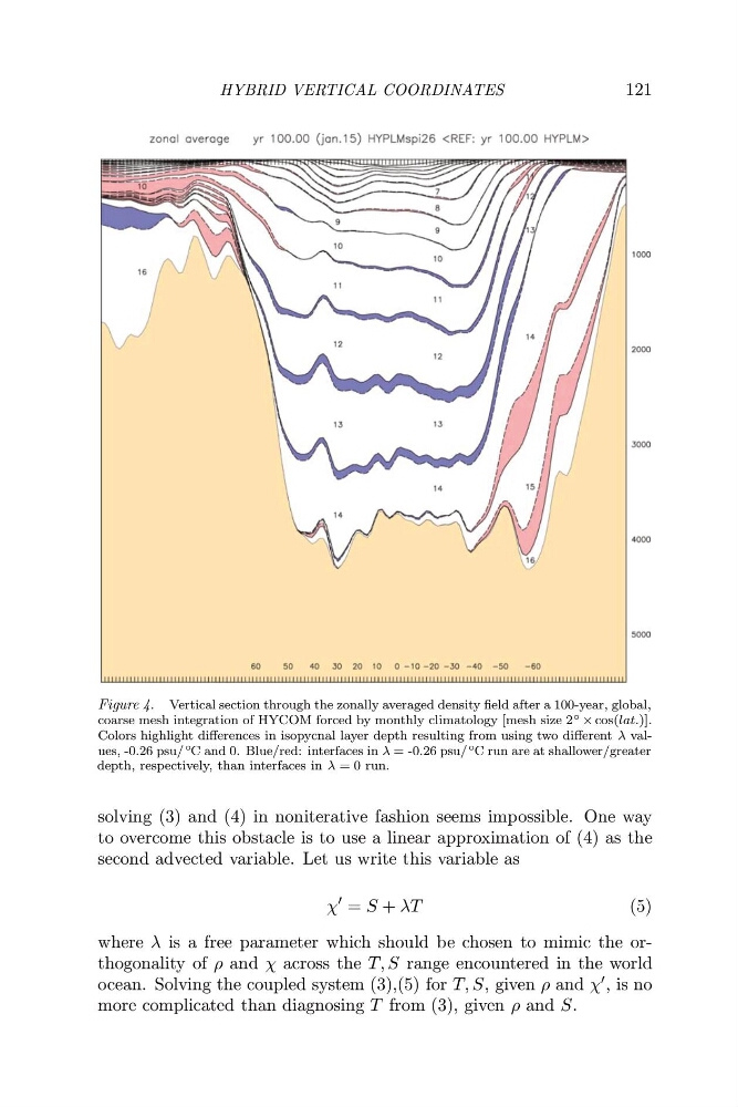
Figure 4. Vertical section through the zonally averaged density field after a 100-year, global,
coarse mesh integration of HYCOM forced by monthly climatology [mesh size 2 ◦ × cos(lat.)].
Colors highlight differences in isopycnal layer depth resulting from using two different λ values, -0.26 psu/ ◦ C and 0. Blue/red: interfaces in λ = -0.26 psu/ ◦ C run are at shallower/greater
depth, respectively, than interfaces in λ = 0 run.
solving (3) and (4) in noniterative fashion seems impossible. One way
to overcome this obstacle is to use a linear approximation of (4) as the
second advected variable. Let us write this variable as
χ
= S + λT
(5)
where λ is a free parameter which should be chosen to mimic the orthogonality of ρ and χ across the T, S range encountered in the world
ocean. Solving the coupled system (3),(5) for T, S, given ρ and χ , is no
more complicated than diagnosing T from (3), given ρ and S.
121
Figure 4. Vertical section through the zonally averaged density field after a 100-year, global,
coarse mesh integration of HYCOM forced by monthly climatology [mesh size 2 ◦ × cos(lat.)].
Colors highlight differences in isopycnal layer depth resulting from using two different λ values, -0.26 psu/ ◦ C and 0. Blue/red: interfaces in λ = -0.26 psu/ ◦ C run are at shallower/greater
depth, respectively, than interfaces in λ = 0 run.
solving (3) and (4) in noniterative fashion seems impossible. One way
to overcome this obstacle is to use a linear approximation of (4) as the
second advected variable. Let us write this variable as
χ
= S + λT
(5)
where λ is a free parameter which should be chosen to mimic the orthogonality of ρ and χ across the T, S range encountered in the world
ocean. Solving the coupled system (3),(5) for T, S, given ρ and χ , is no
more complicated than diagnosing T from (3), given ρ and S.