

3.5 Exercise 3: Short Surface Gravity Waves
33
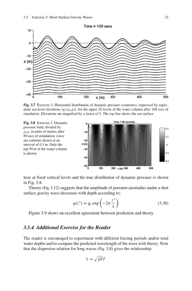
Fig. 3.7 Exercise 3. Horizontal distribution of dynamic pressure (contours), expressed by equivalent sea-level elevations (q/(ρ o g)), for the upper 20 levels of the water column after 100 secs of
simulation. Elevations are magnified by a factor of 5. The top line shows the sea surface
Fig. 3.8 Exercise 3. Dynamic
pressure field, divided by
ρ o g, in units of metres after
80 secs of simulation. Lines
are contours drawn at an
interval of 0.1 m. Only the
top 50 m of the water column
is shown
here at fixed vertical levels and the true distribution of dynamic pressure is shown
in Fig. 3.8.
Theory (Eq. 3.12) suggests that the amplitude of pressure anomalies under a shot
surface gravity wave decreases with depth according to:
q(z
∗ ) = q s exp
−2π
z
∗
λ
(3.36)
Figure 3.9 shows an excellent agreement between prediction and theory.
3.5.4 Additional Exercise for the Reader
The reader is encouraged to experiment with different forcing periods and/or total
water depths and to compare the predicted wavelength of the wave with theory. Note
that the dispersion relation for long waves (Eq. 3.8) gives the relationship:
λ =
ghT
33
Fig. 3.7 Exercise 3. Horizontal distribution of dynamic pressure (contours), expressed by equivalent sea-level elevations (q/(ρ o g)), for the upper 20 levels of the water column after 100 secs of
simulation. Elevations are magnified by a factor of 5. The top line shows the sea surface
Fig. 3.8 Exercise 3. Dynamic
pressure field, divided by
ρ o g, in units of metres after
80 secs of simulation. Lines
are contours drawn at an
interval of 0.1 m. Only the
top 50 m of the water column
is shown
here at fixed vertical levels and the true distribution of dynamic pressure is shown
in Fig. 3.8.
Theory (Eq. 3.12) suggests that the amplitude of pressure anomalies under a shot
surface gravity wave decreases with depth according to:
q(z
∗ ) = q s exp
−2π
z
∗
λ
(3.36)
Figure 3.9 shows an excellent agreement between prediction and theory.
3.5.4 Additional Exercise for the Reader
The reader is encouraged to experiment with different forcing periods and/or total
water depths and to compare the predicted wavelength of the wave with theory. Note
that the dispersion relation for long waves (Eq. 3.8) gives the relationship:
λ =
ghT