

32
3 Basics of Nonhydrostatic Modelling
where h max is the maximum total water depth encountered in the model domain.
This is known as Courant-Friedrichs-Lewy condition or CFL condition for surface
gravity waves (Courant et al., 1928).
3.5 Exercise 3: Short Surface Gravity Waves
3.5.1 Aim
The aim of this exercise is to simulate the progression of short surface gravity waves
in an ocean uniform in density.
3.5.2 Task Description
The task is to construct a FORTRAN 95 simulation code based on the nonhydrostatic finite-difference equations outlined in the previous section. Consider a
channel, 500 m in length and 100 m deep, resolved by grid spacings of Δx = 5 m
and Δz = 2 m. Both ends of the channel are closed. Zero-gradient conditions for
dynamic pressure are applied at these boundaries. These boundary conditions imply
that pressure surfaces intersect the boundary at a right angle, which is consistent
with the condition of vanishing normal flow.
Forcing consists of oscillatory sea level variations of 1 m in amplitude on a period
of 8 s, prescribed near the left boundary. According to the dispersion relation of short
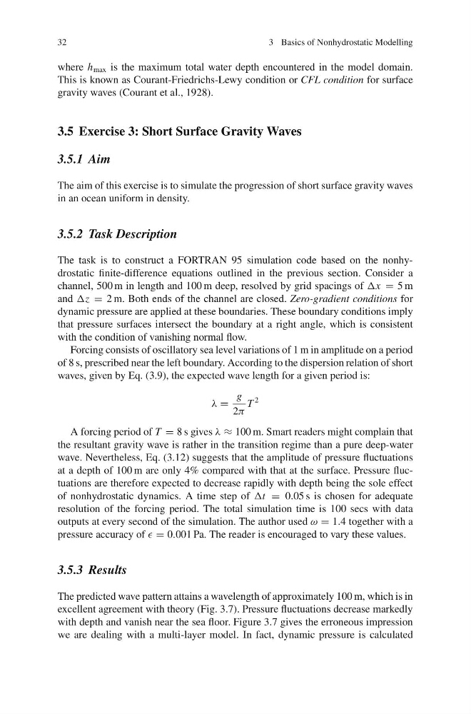
waves, given by Eq. (3.9), the expected wave length for a given period is:
λ =
g
2π
T
2
A forcing period of T = 8 s gives λ ≈ 100 m. Smart readers might complain that
the resultant gravity wave is rather in the transition regime than a pure deep-water
wave. Nevertheless, Eq. (3.12) suggests that the amplitude of pressure fluctuations
at a depth of 100 m are only 4% compared with that at the surface. Pressure fluctuations are therefore expected to decrease rapidly with depth being the sole effect
of nonhydrostatic dynamics. A time step of Δt = 0.05 s is chosen for adequate
resolution of the forcing period. The total simulation time is 100 secs with data
outputs at every second of the simulation. The author used ω = 1.4 together with a
pressure accuracy of = 0.001 Pa. The reader is encouraged to vary these values.
3.5.3 Results
The predicted wave pattern attains a wavelength of approximately 100 m, which is in
excellent agreement with theory (Fig. 3.7). Pressure fluctuations decrease markedly
with depth and vanish near the sea floor. Figure 3.7 gives the erroneous impression
we are dealing with a multi-layer model. In fact, dynamic pressure is calculated
3 Basics of Nonhydrostatic Modelling
where h max is the maximum total water depth encountered in the model domain.
This is known as Courant-Friedrichs-Lewy condition or CFL condition for surface
gravity waves (Courant et al., 1928).
3.5 Exercise 3: Short Surface Gravity Waves
3.5.1 Aim
The aim of this exercise is to simulate the progression of short surface gravity waves
in an ocean uniform in density.
3.5.2 Task Description
The task is to construct a FORTRAN 95 simulation code based on the nonhydrostatic finite-difference equations outlined in the previous section. Consider a
channel, 500 m in length and 100 m deep, resolved by grid spacings of Δx = 5 m
and Δz = 2 m. Both ends of the channel are closed. Zero-gradient conditions for
dynamic pressure are applied at these boundaries. These boundary conditions imply
that pressure surfaces intersect the boundary at a right angle, which is consistent
with the condition of vanishing normal flow.
Forcing consists of oscillatory sea level variations of 1 m in amplitude on a period
of 8 s, prescribed near the left boundary. According to the dispersion relation of short
waves, given by Eq. (3.9), the expected wave length for a given period is:
λ =
g
2π
T
2
A forcing period of T = 8 s gives λ ≈ 100 m. Smart readers might complain that
the resultant gravity wave is rather in the transition regime than a pure deep-water
wave. Nevertheless, Eq. (3.12) suggests that the amplitude of pressure fluctuations
at a depth of 100 m are only 4% compared with that at the surface. Pressure fluctuations are therefore expected to decrease rapidly with depth being the sole effect
of nonhydrostatic dynamics. A time step of Δt = 0.05 s is chosen for adequate
resolution of the forcing period. The total simulation time is 100 secs with data
outputs at every second of the simulation. The author used ω = 1.4 together with a
pressure accuracy of = 0.001 Pa. The reader is encouraged to vary these values.
3.5.3 Results
The predicted wave pattern attains a wavelength of approximately 100 m, which is in
excellent agreement with theory (Fig. 3.7). Pressure fluctuations decrease markedly
with depth and vanish near the sea floor. Figure 3.7 gives the erroneous impression
we are dealing with a multi-layer model. In fact, dynamic pressure is calculated