

2.2 The Surface Ekman Layer
11
2.2 The Surface Ekman Layer
2.2.1 Boundary-Layer Equations
This section explores the dynamics of frictional boundary layers in the ocean, called
Ekman layers (Ekman, 1905). For simplicity, we assume horizontal homogeneity of
all variables and an ocean of uniform density, so that the Navier-Stokes equations
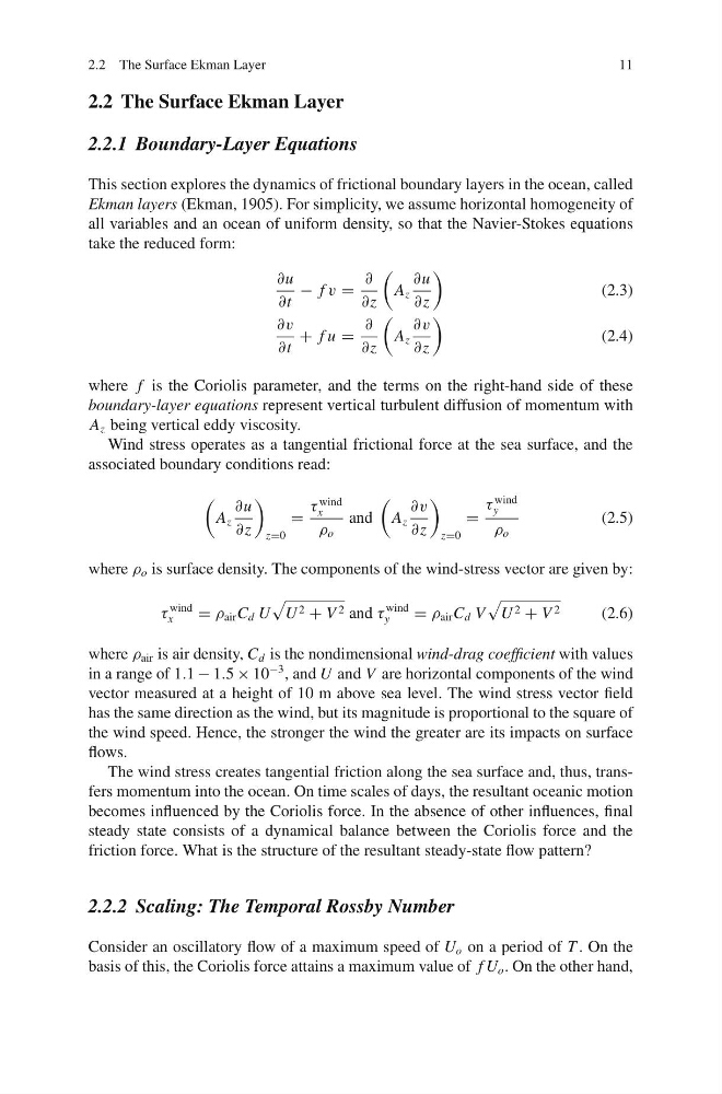
take the reduced form:
∂u
∂t
− f v =
∂
∂z
A z
∂u
∂z
(2.3)
∂v
∂t
+ f u =
∂
∂z
A z
∂v
∂z
(2.4)
where f is the Coriolis parameter, and the terms on the right-hand side of these
boundary-layer equations represent vertical turbulent diffusion of momentum with
A z being vertical eddy viscosity.
Wind stress operates as a tangential frictional force at the sea surface, and the
associated boundary conditions read:
A z
∂u
∂z
z=0
=
τ
wind
x
ρ o
and
A z
∂v
∂z
z=0
=
τ
wind
y
ρ o
(2.5)
where ρ o is surface density. The components of the wind-stress vector are given by:
τ
wind
x
= ρ air C d U
U 2 + V 2 and τ
wind
y
= ρ air C d V
U 2 + V 2
(2.6)
where ρ air is air density, C d is the nondimensional wind-drag coefficient with values
in a range of 1.1 − 1.5 × 10
−3 , and U and V are horizontal components of the wind
vector measured at a height of 10 m above sea level. The wind stress vector field
has the same direction as the wind, but its magnitude is proportional to the square of
the wind speed. Hence, the stronger the wind the greater are its impacts on surface
flows.
The wind stress creates tangential friction along the sea surface and, thus, transfers momentum into the ocean. On time scales of days, the resultant oceanic motion
becomes influenced by the Coriolis force. In the absence of other influences, final
steady state consists of a dynamical balance between the Coriolis force and the
friction force. What is the structure of the resultant steady-state flow pattern?
2.2.2 Scaling: The Temporal Rossby Number
Consider an oscillatory flow of a maximum speed of U o on a period of T . On the
basis of this, the Coriolis force attains a maximum value of f U o . On the other hand,
11
2.2 The Surface Ekman Layer
2.2.1 Boundary-Layer Equations
This section explores the dynamics of frictional boundary layers in the ocean, called
Ekman layers (Ekman, 1905). For simplicity, we assume horizontal homogeneity of
all variables and an ocean of uniform density, so that the Navier-Stokes equations
take the reduced form:
∂u
∂t
− f v =
∂
∂z
A z
∂u
∂z
(2.3)
∂v
∂t
+ f u =
∂
∂z
A z
∂v
∂z
(2.4)
where f is the Coriolis parameter, and the terms on the right-hand side of these
boundary-layer equations represent vertical turbulent diffusion of momentum with
A z being vertical eddy viscosity.
Wind stress operates as a tangential frictional force at the sea surface, and the
associated boundary conditions read:
A z
∂u
∂z
z=0
=
τ
wind
x
ρ o
and
A z
∂v
∂z
z=0
=
τ
wind
y
ρ o
(2.5)
where ρ o is surface density. The components of the wind-stress vector are given by:
τ
wind
x
= ρ air C d U
U 2 + V 2 and τ
wind
y
= ρ air C d V
U 2 + V 2
(2.6)
where ρ air is air density, C d is the nondimensional wind-drag coefficient with values
in a range of 1.1 − 1.5 × 10
−3 , and U and V are horizontal components of the wind
vector measured at a height of 10 m above sea level. The wind stress vector field
has the same direction as the wind, but its magnitude is proportional to the square of
the wind speed. Hence, the stronger the wind the greater are its impacts on surface
flows.
The wind stress creates tangential friction along the sea surface and, thus, transfers momentum into the ocean. On time scales of days, the resultant oceanic motion
becomes influenced by the Coriolis force. In the absence of other influences, final
steady state consists of a dynamical balance between the Coriolis force and the
friction force. What is the structure of the resultant steady-state flow pattern?
2.2.2 Scaling: The Temporal Rossby Number
Consider an oscillatory flow of a maximum speed of U o on a period of T . On the
basis of this, the Coriolis force attains a maximum value of f U o . On the other hand,