

10
2 1D Models of Ekman Layers
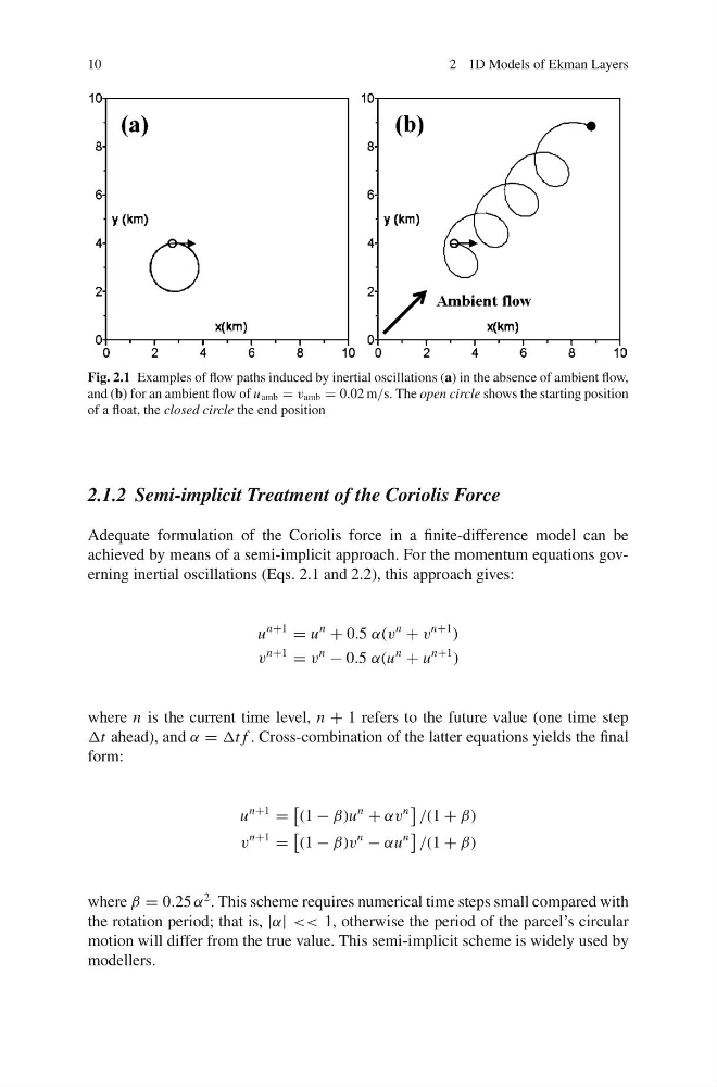
Fig. 2.1 Examples of flow paths induced by inertial oscillations (a) in the absence of ambient flow,
and (b) for an ambient flow of u amb = v amb = 0.02 m/s. The open circle shows the starting position
of a float, the closed circle the end position
2.1.2 Semi-implicit Treatment of the Coriolis Force
Adequate formulation of the Coriolis force in a finite-difference model can be
achieved by means of a semi-implicit approach. For the momentum equations governing inertial oscillations (Eqs. 2.1 and 2.2), this approach gives:
u
n+1
= u
n
+ 0.5 α(v
n
+ v
n+1 )
v
n+1
= v
n
− 0.5 α(u
n
+ u
n+1 )
where n is the current time level, n + 1 refers to the future value (one time step
Δt ahead), and α = Δt f . Cross-combination of the latter equations yields the final
form:
u
n+1
=
(1 − β)u
n
+ αv
n
/(1 + β)
v
n+1
=
(1 − β)v
n
− αu
n
/(1 + β)
where β = 0.25 α
2 . This scheme requires numerical time steps small compared with
the rotation period; that is, |α| << 1, otherwise the period of the parcel’s circular
motion will differ from the true value. This semi-implicit scheme is widely used by
modellers.
2 1D Models of Ekman Layers
Fig. 2.1 Examples of flow paths induced by inertial oscillations (a) in the absence of ambient flow,
and (b) for an ambient flow of u amb = v amb = 0.02 m/s. The open circle shows the starting position
of a float, the closed circle the end position
2.1.2 Semi-implicit Treatment of the Coriolis Force
Adequate formulation of the Coriolis force in a finite-difference model can be
achieved by means of a semi-implicit approach. For the momentum equations governing inertial oscillations (Eqs. 2.1 and 2.2), this approach gives:
u
n+1
= u
n
+ 0.5 α(v
n
+ v
n+1 )
v
n+1
= v
n
− 0.5 α(u
n
+ u
n+1 )
where n is the current time level, n + 1 refers to the future value (one time step
Δt ahead), and α = Δt f . Cross-combination of the latter equations yields the final
form:
u
n+1
=
(1 − β)u
n
+ αv
n
/(1 + β)
v
n+1
=
(1 − β)v
n
− αu
n
/(1 + β)
where β = 0.25 α
2 . This scheme requires numerical time steps small compared with
the rotation period; that is, |α| << 1, otherwise the period of the parcel’s circular
motion will differ from the true value. This semi-implicit scheme is widely used by
modellers.