

5.13 Advanced Lateral Boundary Conditions
169
5.13.6 Radiation Conditions
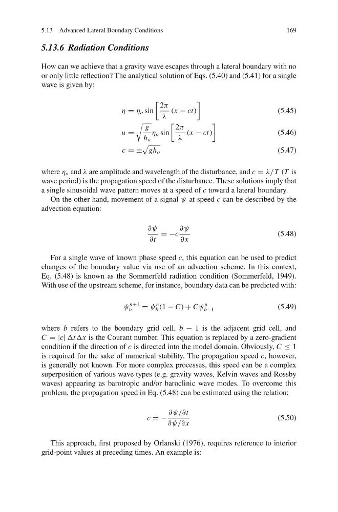
How can we achieve that a gravity wave escapes through a lateral boundary with no
or only little reflection? The analytical solution of Eqs. (5.40) and (5.41) for a single
wave is given by:
η = η o sin
2π
λ
(x − ct)
(5.45)
u =
g
h o
η o sin
2π
λ
(x − ct)
(5.46)
c = ±
gh o
(5.47)
where η o and λ are amplitude and wavelength of the disturbance, and c = λ/T (T is
wave period) is the propagation speed of the disturbance. These solutions imply that
a single sinusoidal wave pattern moves at a speed of c toward a lateral boundary.
On the other hand, movement of a signal ψ at speed c can be described by the
advection equation:
∂ψ
∂t
= −c
∂ψ
∂ x
(5.48)
For a single wave of known phase speed c, this equation can be used to predict
changes of the boundary value via use of an advection scheme. In this context,
Eq. (5.48) is known as the Sommerfeld radiation condition (Sommerfeld, 1949).
With use of the upstream scheme, for instance, boundary data can be predicted with:
ψ
n+1
b
= ψ
n
b (1 − C) + Cψ
n
b−1
(5.49)
where b refers to the boundary grid cell, b − 1 is the adjacent grid cell, and
C = |c| ΔtΔx is the Courant number. This equation is replaced by a zero-gradient
condition if the direction of c is directed into the model domain. Obviously, C ≤ 1
is required for the sake of numerical stability. The propagation speed c, however,
is generally not known. For more complex processes, this speed can be a complex
superposition of various wave types (e.g. gravity waves, Kelvin waves and Rossby
waves) appearing as barotropic and/or baroclinic wave modes. To overcome this
problem, the propagation speed in Eq. (5.48) can be estimated using the relation:
c = −
∂ψ/∂t
∂ψ/∂x
(5.50)
This approach, first proposed by Orlanski (1976), requires reference to interior
grid-point values at preceding times. An example is:
169
5.13.6 Radiation Conditions
How can we achieve that a gravity wave escapes through a lateral boundary with no
or only little reflection? The analytical solution of Eqs. (5.40) and (5.41) for a single
wave is given by:
η = η o sin
2π
λ
(x − ct)
(5.45)
u =
g
h o
η o sin
2π
λ
(x − ct)
(5.46)
c = ±
gh o
(5.47)
where η o and λ are amplitude and wavelength of the disturbance, and c = λ/T (T is
wave period) is the propagation speed of the disturbance. These solutions imply that
a single sinusoidal wave pattern moves at a speed of c toward a lateral boundary.
On the other hand, movement of a signal ψ at speed c can be described by the
advection equation:
∂ψ
∂t
= −c
∂ψ
∂ x
(5.48)
For a single wave of known phase speed c, this equation can be used to predict
changes of the boundary value via use of an advection scheme. In this context,
Eq. (5.48) is known as the Sommerfeld radiation condition (Sommerfeld, 1949).
With use of the upstream scheme, for instance, boundary data can be predicted with:
ψ
n+1
b
= ψ
n
b (1 − C) + Cψ
n
b−1
(5.49)
where b refers to the boundary grid cell, b − 1 is the adjacent grid cell, and
C = |c| ΔtΔx is the Courant number. This equation is replaced by a zero-gradient
condition if the direction of c is directed into the model domain. Obviously, C ≤ 1
is required for the sake of numerical stability. The propagation speed c, however,
is generally not known. For more complex processes, this speed can be a complex
superposition of various wave types (e.g. gravity waves, Kelvin waves and Rossby
waves) appearing as barotropic and/or baroclinic wave modes. To overcome this
problem, the propagation speed in Eq. (5.48) can be estimated using the relation:
c = −
∂ψ/∂t
∂ψ/∂x
(5.50)
This approach, first proposed by Orlanski (1976), requires reference to interior
grid-point values at preceding times. An example is: