

168
5 3D Level Modelling
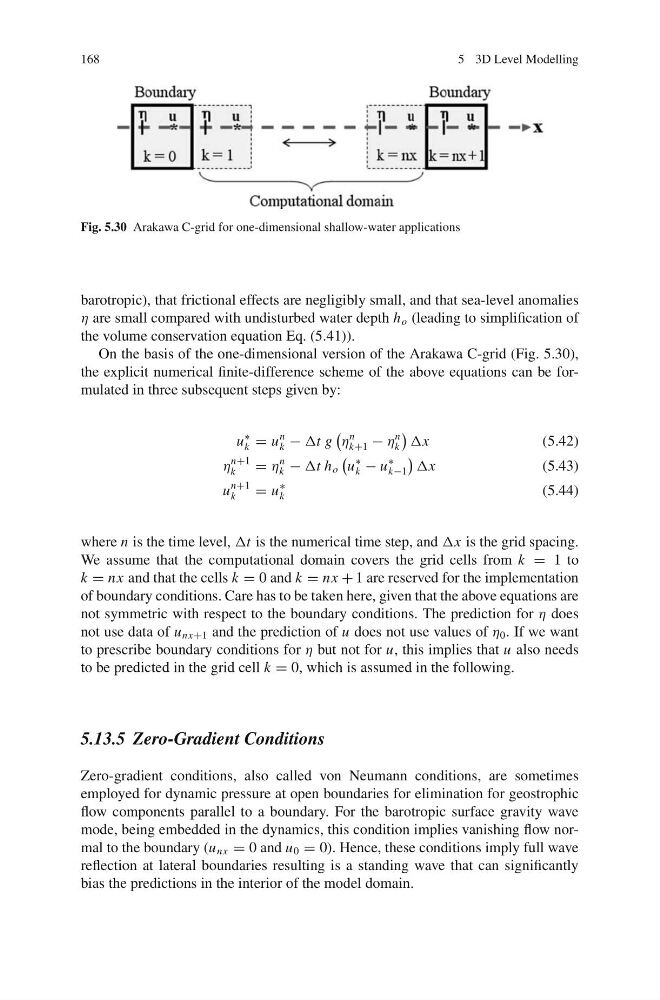
Fig. 5.30 Arakawa C-grid for one-dimensional shallow-water applications
barotropic), that frictional effects are negligibly small, and that sea-level anomalies
η are small compared with undisturbed water depth h o (leading to simplification of
the volume conservation equation Eq. (5.41)).
On the basis of the one-dimensional version of the Arakawa C-grid (Fig. 5.30),
the explicit numerical finite-difference scheme of the above equations can be formulated in three subsequent steps given by:
u
∗
k = u
n
k − Δt g
η
n
k+1 − η
n
k
Δx
(5.42)
η
n+1
k
= η
n
k − Δt h o
u
∗
k − u
∗
k−1
Δx
(5.43)
u
n+1
k
= u
∗
k
(5.44)
where n is the time level, Δt is the numerical time step, and Δx is the grid spacing.
We assume that the computational domain covers the grid cells from k = 1 to
k = nx and that the cells k = 0 and k = nx + 1 are reserved for the implementation
of boundary conditions. Care has to be taken here, given that the above equations are
not symmetric with respect to the boundary conditions. The prediction for η does
not use data of u nx+1 and the prediction of u does not use values of η 0 . If we want
to prescribe boundary conditions for η but not for u, this implies that u also needs
to be predicted in the grid cell k = 0, which is assumed in the following.
5.13.5 Zero-Gradient Conditions
Zero-gradient conditions, also called von Neumann conditions, are sometimes
employed for dynamic pressure at open boundaries for elimination for geostrophic
flow components parallel to a boundary. For the barotropic surface gravity wave
mode, being embedded in the dynamics, this condition implies vanishing flow normal to the boundary (u nx = 0 and u 0 = 0). Hence, these conditions imply full wave
reflection at lateral boundaries resulting is a standing wave that can significantly
bias the predictions in the interior of the model domain.
5 3D Level Modelling
Fig. 5.30 Arakawa C-grid for one-dimensional shallow-water applications
barotropic), that frictional effects are negligibly small, and that sea-level anomalies
η are small compared with undisturbed water depth h o (leading to simplification of
the volume conservation equation Eq. (5.41)).
On the basis of the one-dimensional version of the Arakawa C-grid (Fig. 5.30),
the explicit numerical finite-difference scheme of the above equations can be formulated in three subsequent steps given by:
u
∗
k = u
n
k − Δt g
η
n
k+1 − η
n
k
Δx
(5.42)
η
n+1
k
= η
n
k − Δt h o
u
∗
k − u
∗
k−1
Δx
(5.43)
u
n+1
k
= u
∗
k
(5.44)
where n is the time level, Δt is the numerical time step, and Δx is the grid spacing.
We assume that the computational domain covers the grid cells from k = 1 to
k = nx and that the cells k = 0 and k = nx + 1 are reserved for the implementation
of boundary conditions. Care has to be taken here, given that the above equations are
not symmetric with respect to the boundary conditions. The prediction for η does
not use data of u nx+1 and the prediction of u does not use values of η 0 . If we want
to prescribe boundary conditions for η but not for u, this implies that u also needs
to be predicted in the grid cell k = 0, which is assumed in the following.
5.13.5 Zero-Gradient Conditions
Zero-gradient conditions, also called von Neumann conditions, are sometimes
employed for dynamic pressure at open boundaries for elimination for geostrophic
flow components parallel to a boundary. For the barotropic surface gravity wave
mode, being embedded in the dynamics, this condition implies vanishing flow normal to the boundary (u nx = 0 and u 0 = 0). Hence, these conditions imply full wave
reflection at lateral boundaries resulting is a standing wave that can significantly
bias the predictions in the interior of the model domain.