

170
5 3D Level Modelling
C =
ψ
n
b−1 − ψ
n−1
b−1
ψ
n−1
b−2 − ψ
n−1
b−1
(5.51)
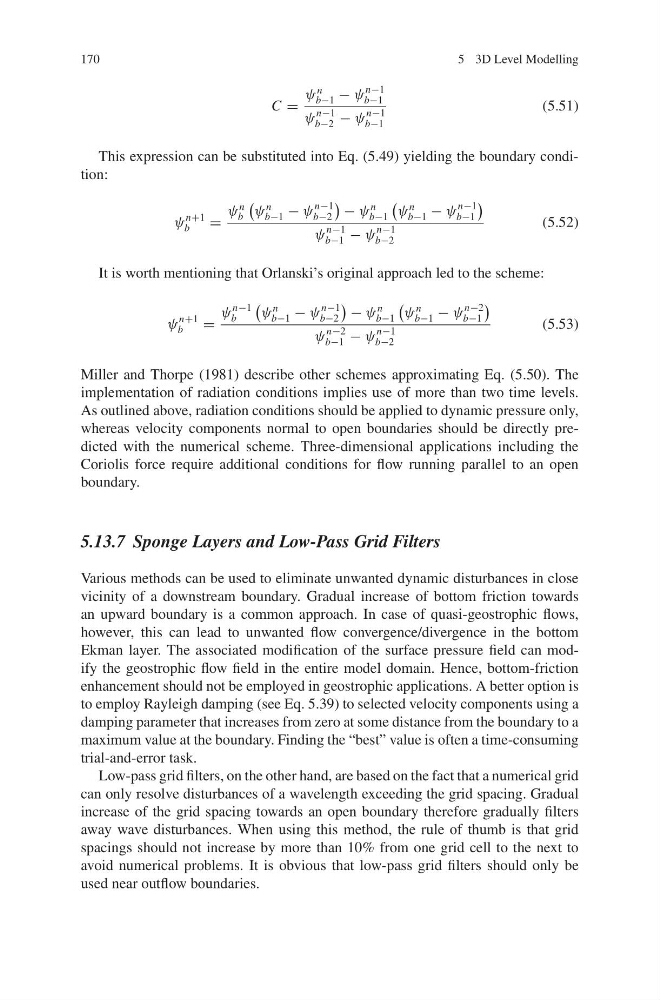
This expression can be substituted into Eq. (5.49) yielding the boundary condition:
ψ
n+1
b
=
ψ
n
b
ψ
n
b−1 − ψ
n−1
b−2
− ψ
n
b−1
ψ
n
b−1 − ψ
n−1
b−1
ψ
n−1
b−1 − ψ
n−1
b−2
(5.52)
It is worth mentioning that Orlanski’s original approach led to the scheme:
ψ
n+1
b
=
ψ
n−1
b
ψ
n
b−1 − ψ
n−1
b−2
− ψ
n
b−1
ψ
n
b−1 − ψ
n−2
b−1
ψ
n−2
b−1 − ψ
n−1
b−2
(5.53)
Miller and Thorpe (1981) describe other schemes approximating Eq. (5.50). The
implementation of radiation conditions implies use of more than two time levels.
As outlined above, radiation conditions should be applied to dynamic pressure only,
whereas velocity components normal to open boundaries should be directly predicted with the numerical scheme. Three-dimensional applications including the
Coriolis force require additional conditions for flow running parallel to an open
boundary.
5.13.7 Sponge Layers and Low-Pass Grid Filters
Various methods can be used to eliminate unwanted dynamic disturbances in close
vicinity of a downstream boundary. Gradual increase of bottom friction towards
an upward boundary is a common approach. In case of quasi-geostrophic flows,
however, this can lead to unwanted flow convergence/divergence in the bottom
Ekman layer. The associated modification of the surface pressure field can modify the geostrophic flow field in the entire model domain. Hence, bottom-friction
enhancement should not be employed in geostrophic applications. A better option is
to employ Rayleigh damping (see Eq. 5.39) to selected velocity components using a
damping parameter that increases from zero at some distance from the boundary to a
maximum value at the boundary. Finding the “best” value is often a time-consuming
trial-and-error task.
Low-pass grid filters, on the other hand, are based on the fact that a numerical grid
can only resolve disturbances of a wavelength exceeding the grid spacing. Gradual
increase of the grid spacing towards an open boundary therefore gradually filters
away wave disturbances. When using this method, the rule of thumb is that grid
spacings should not increase by more than 10% from one grid cell to the next to
avoid numerical problems. It is obvious that low-pass grid filters should only be
used near outflow boundaries.
5 3D Level Modelling
C =
ψ
n
b−1 − ψ
n−1
b−1
ψ
n−1
b−2 − ψ
n−1
b−1
(5.51)
This expression can be substituted into Eq. (5.49) yielding the boundary condition:
ψ
n+1
b
=
ψ
n
b
ψ
n
b−1 − ψ
n−1
b−2
− ψ
n
b−1
ψ
n
b−1 − ψ
n−1
b−1
ψ
n−1
b−1 − ψ
n−1
b−2
(5.52)
It is worth mentioning that Orlanski’s original approach led to the scheme:
ψ
n+1
b
=
ψ
n−1
b
ψ
n
b−1 − ψ
n−1
b−2
− ψ
n
b−1
ψ
n
b−1 − ψ
n−2
b−1
ψ
n−2
b−1 − ψ
n−1
b−2
(5.53)
Miller and Thorpe (1981) describe other schemes approximating Eq. (5.50). The
implementation of radiation conditions implies use of more than two time levels.
As outlined above, radiation conditions should be applied to dynamic pressure only,
whereas velocity components normal to open boundaries should be directly predicted with the numerical scheme. Three-dimensional applications including the
Coriolis force require additional conditions for flow running parallel to an open
boundary.
5.13.7 Sponge Layers and Low-Pass Grid Filters
Various methods can be used to eliminate unwanted dynamic disturbances in close
vicinity of a downstream boundary. Gradual increase of bottom friction towards
an upward boundary is a common approach. In case of quasi-geostrophic flows,
however, this can lead to unwanted flow convergence/divergence in the bottom
Ekman layer. The associated modification of the surface pressure field can modify the geostrophic flow field in the entire model domain. Hence, bottom-friction
enhancement should not be employed in geostrophic applications. A better option is
to employ Rayleigh damping (see Eq. 5.39) to selected velocity components using a
damping parameter that increases from zero at some distance from the boundary to a
maximum value at the boundary. Finding the “best” value is often a time-consuming
trial-and-error task.
Low-pass grid filters, on the other hand, are based on the fact that a numerical grid
can only resolve disturbances of a wavelength exceeding the grid spacing. Gradual
increase of the grid spacing towards an open boundary therefore gradually filters
away wave disturbances. When using this method, the rule of thumb is that grid
spacings should not increase by more than 10% from one grid cell to the next to
avoid numerical problems. It is obvious that low-pass grid filters should only be
used near outflow boundaries.