

160
5 3D Level Modelling
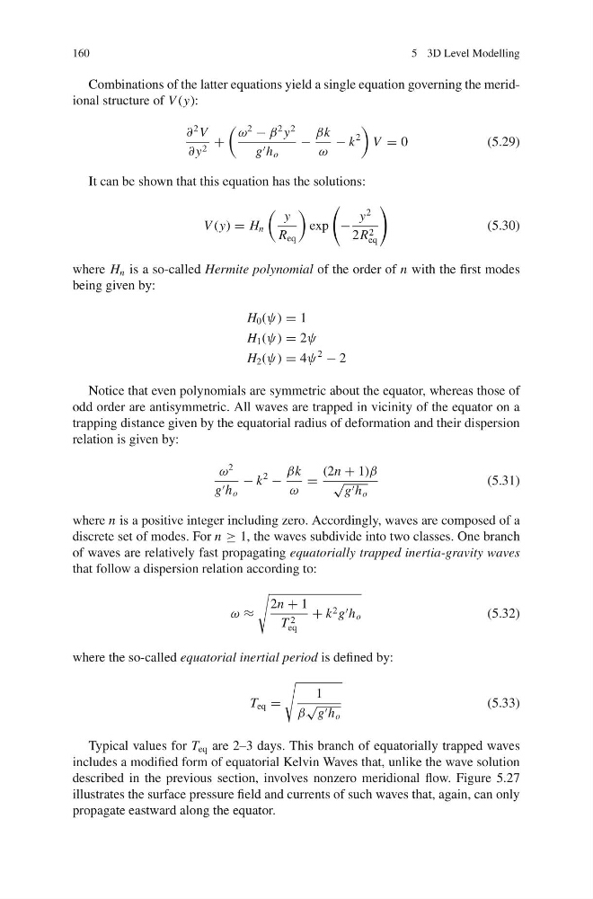
Combinations of the latter equations yield a single equation governing the meridional structure of V (y):
∂
2 V
∂ y 2 +
ω
2
− β
2 y
2
g h o
−
βk
ω
− k
2
V = 0
(5.29)
It can be shown that this equation has the solutions:
V (y) = H n
y
R eq
exp
−
y
2
2R 2
eq
(5.30)
where H n is a so-called Hermite polynomial of the order of n with the first modes
being given by:
H 0 (ψ) = 1
H 1 (ψ) = 2ψ
H 2 (ψ) = 4ψ
2
− 2
Notice that even polynomials are symmetric about the equator, whereas those of
odd order are antisymmetric. All waves are trapped in vicinity of the equator on a
trapping distance given by the equatorial radius of deformation and their dispersion
relation is given by:
ω
2
g h o
− k
2
−
βk
ω
=
(2n + 1)β
√
g h o
(5.31)
where n is a positive integer including zero. Accordingly, waves are composed of a
discrete set of modes. For n ≥ 1, the waves subdivide into two classes. One branch
of waves are relatively fast propagating equatorially trapped inertia-gravity waves
that follow a dispersion relation according to:
ω ≈
2n + 1
T 2
eq
+ k 2 g h o
(5.32)
where the so-called equatorial inertial period is defined by:
T eq =
1
β
√
g h o
(5.33)
Typical values for T eq are 2–3 days. This branch of equatorially trapped waves
includes a modified form of equatorial Kelvin Waves that, unlike the wave solution
described in the previous section, involves nonzero meridional flow. Figure 5.27
illustrates the surface pressure field and currents of such waves that, again, can only
propagate eastward along the equator.
5 3D Level Modelling
Combinations of the latter equations yield a single equation governing the meridional structure of V (y):
∂
2 V
∂ y 2 +
ω
2
− β
2 y
2
g h o
−
βk
ω
− k
2
V = 0
(5.29)
It can be shown that this equation has the solutions:
V (y) = H n
y
R eq
exp
−
y
2
2R 2
eq
(5.30)
where H n is a so-called Hermite polynomial of the order of n with the first modes
being given by:
H 0 (ψ) = 1
H 1 (ψ) = 2ψ
H 2 (ψ) = 4ψ
2
− 2
Notice that even polynomials are symmetric about the equator, whereas those of
odd order are antisymmetric. All waves are trapped in vicinity of the equator on a
trapping distance given by the equatorial radius of deformation and their dispersion
relation is given by:
ω
2
g h o
− k
2
−
βk
ω
=
(2n + 1)β
√
g h o
(5.31)
where n is a positive integer including zero. Accordingly, waves are composed of a
discrete set of modes. For n ≥ 1, the waves subdivide into two classes. One branch
of waves are relatively fast propagating equatorially trapped inertia-gravity waves
that follow a dispersion relation according to:
ω ≈
2n + 1
T 2
eq
+ k 2 g h o
(5.32)
where the so-called equatorial inertial period is defined by:
T eq =
1
β
√
g h o
(5.33)
Typical values for T eq are 2–3 days. This branch of equatorially trapped waves
includes a modified form of equatorial Kelvin Waves that, unlike the wave solution
described in the previous section, involves nonzero meridional flow. Figure 5.27
illustrates the surface pressure field and currents of such waves that, again, can only
propagate eastward along the equator.