

158
5 3D Level Modelling
5.10 Equatorial Waves
5.10.1 Background
The existence of the equator gives rise to special kinds of oceanic waves that otherwise would not exist. The dynamical reason for such waves is that the Coriolis
force changes sign across the equator, giving rise to equatorial inertial oscillations
described in the previous section. However, there are other wave types existing in
vicinity of the equator. The most basic equations describing these waves rely on
the reduced-gravity concept for a two-layer ocean (e.g. Cushman-Roisin, 1994)
in which the bottom layer always adjusts such that the lateral flow in this layer
vanishes. If we describe the thickness of the upper layer as the sum of a constant
part h o and a fluctuating part η
∗ , the reduced-gravity concept leads to the following
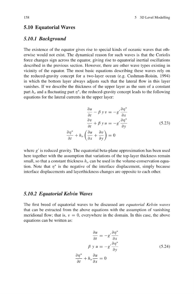
equations for the lateral currents in the upper layer:
∂u
∂t
− β y v = −g
∂η
∗
∂ x
∂v
∂t
+ β y u = −g
∂η
∗
∂ y
(5.23)
∂η
∗
∂t
+ h o
∂u
∂ x
+
∂v
∂ y
= 0
where g
is reduced gravity. The equatorial beta-plane approximation has been used
here together with the assumption that variations of the top-layer thickness remain
small, so that a constant thickness h o can be used in the volume-conservation equation. Note that η
∗ is the negative of the interface displacement, simply because
interface displacements and layerthickness changes are opposite to each other.
5.10.2 Equatorial Kelvin Waves
The first breed of equatorial waves to be discussed are equatorial Kelvin waves
that can be extracted from the above equations with the assumption of vanishing
meridional flow; that is, v = 0, everywhere in the domain. In this case, the above
equations can be written as:
∂u
∂t
= −g
∂η
∗
∂ x
β y u = −g
∂η
∗
∂ y
(5.24)
∂η
∗
∂t
+ h o
∂u
∂ x
= 0
5 3D Level Modelling
5.10 Equatorial Waves
5.10.1 Background
The existence of the equator gives rise to special kinds of oceanic waves that otherwise would not exist. The dynamical reason for such waves is that the Coriolis
force changes sign across the equator, giving rise to equatorial inertial oscillations
described in the previous section. However, there are other wave types existing in
vicinity of the equator. The most basic equations describing these waves rely on
the reduced-gravity concept for a two-layer ocean (e.g. Cushman-Roisin, 1994)
in which the bottom layer always adjusts such that the lateral flow in this layer
vanishes. If we describe the thickness of the upper layer as the sum of a constant
part h o and a fluctuating part η
∗ , the reduced-gravity concept leads to the following
equations for the lateral currents in the upper layer:
∂u
∂t
− β y v = −g
∂η
∗
∂ x
∂v
∂t
+ β y u = −g
∂η
∗
∂ y
(5.23)
∂η
∗
∂t
+ h o
∂u
∂ x
+
∂v
∂ y
= 0
where g
is reduced gravity. The equatorial beta-plane approximation has been used
here together with the assumption that variations of the top-layer thickness remain
small, so that a constant thickness h o can be used in the volume-conservation equation. Note that η
∗ is the negative of the interface displacement, simply because
interface displacements and layerthickness changes are opposite to each other.
5.10.2 Equatorial Kelvin Waves
The first breed of equatorial waves to be discussed are equatorial Kelvin waves
that can be extracted from the above equations with the assumption of vanishing
meridional flow; that is, v = 0, everywhere in the domain. In this case, the above
equations can be written as:
∂u
∂t
= −g
∂η
∗
∂ x
β y u = −g
∂η
∗
∂ y
(5.24)
∂η
∗
∂t
+ h o
∂u
∂ x
= 0