

5.6 Exercise 23: Coastal Upwelling in 3D
143
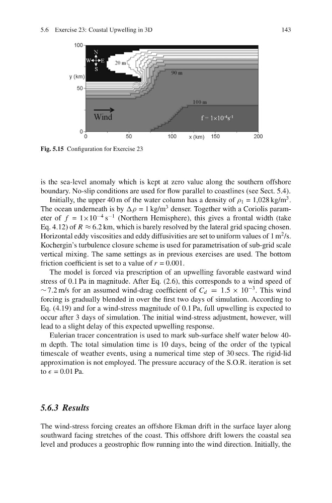
Fig. 5.15 Configuration for Exercise 23
is the sea-level anomaly which is kept at zero value along the southern offshore
boundary. No-slip conditions are used for flow parallel to coastlines (see Sect. 5.4).
Initially, the upper 40 m of the water column has a density of ρ 1 = 1,028 kg/m
3 .
The ocean underneath is by Δρ = 1 kg/m
3 denser. Together with a Coriolis parameter of f = 1×10
−4 s
−1 (Northern Hemisphere), this gives a frontal width (take
Eq. 4.12) of R ≈ 6.2 km, which is barely resolved by the lateral grid spacing chosen.
Horizontal eddy viscosities and eddy diffusivities are set to uniform values of 1 m
2 /s.
Kochergin’s turbulence closure scheme is used for parametrisation of sub-grid scale
vertical mixing. The same settings as in previous exercises are used. The bottom
friction coefficient is set to a value of r = 0.001.
The model is forced via prescription of an upwelling favorable eastward wind
stress of 0.1 Pa in magnitude. After Eq. (2.6), this corresponds to a wind speed of
∼ 7.2 m/s for an assumed wind-drag coefficient of C d = 1.5 × 10
−3 . This wind
forcing is gradually blended in over the first two days of simulation. According to
Eq. (4.19) and for a wind-stress magnitude of 0.1 Pa, full upwelling is expected to
occur after 3 days of simulation. The initial wind-stress adjustment, however, will
lead to a slight delay of this expected upwelling response.
Eulerian tracer concentration is used to mark sub-surface shelf water below 40m depth. The total simulation time is 10 days, being of the order of the typical
timescale of weather events, using a numerical time step of 30 secs. The rigid-lid
approximation is not employed. The pressure accuracy of the S.O.R. iteration is set
to = 0.01 Pa.
5.6.3 Results
The wind-stress forcing creates an offshore Ekman drift in the surface layer along
southward facing stretches of the coast. This offshore drift lowers the coastal sea
level and produces a geostrophic flow running into the wind direction. Initially, the
143
Fig. 5.15 Configuration for Exercise 23
is the sea-level anomaly which is kept at zero value along the southern offshore
boundary. No-slip conditions are used for flow parallel to coastlines (see Sect. 5.4).
Initially, the upper 40 m of the water column has a density of ρ 1 = 1,028 kg/m
3 .
The ocean underneath is by Δρ = 1 kg/m
3 denser. Together with a Coriolis parameter of f = 1×10
−4 s
−1 (Northern Hemisphere), this gives a frontal width (take
Eq. 4.12) of R ≈ 6.2 km, which is barely resolved by the lateral grid spacing chosen.
Horizontal eddy viscosities and eddy diffusivities are set to uniform values of 1 m
2 /s.
Kochergin’s turbulence closure scheme is used for parametrisation of sub-grid scale
vertical mixing. The same settings as in previous exercises are used. The bottom
friction coefficient is set to a value of r = 0.001.
The model is forced via prescription of an upwelling favorable eastward wind
stress of 0.1 Pa in magnitude. After Eq. (2.6), this corresponds to a wind speed of
∼ 7.2 m/s for an assumed wind-drag coefficient of C d = 1.5 × 10
−3 . This wind
forcing is gradually blended in over the first two days of simulation. According to
Eq. (4.19) and for a wind-stress magnitude of 0.1 Pa, full upwelling is expected to
occur after 3 days of simulation. The initial wind-stress adjustment, however, will
lead to a slight delay of this expected upwelling response.
Eulerian tracer concentration is used to mark sub-surface shelf water below 40m depth. The total simulation time is 10 days, being of the order of the typical
timescale of weather events, using a numerical time step of 30 secs. The rigid-lid
approximation is not employed. The pressure accuracy of the S.O.R. iteration is set
to = 0.01 Pa.
5.6.3 Results
The wind-stress forcing creates an offshore Ekman drift in the surface layer along
southward facing stretches of the coast. This offshore drift lowers the coastal sea
level and produces a geostrophic flow running into the wind direction. Initially, the