

Chapter 1
Introduction
Abstract This chapter reviews the Navier-Stokes equations for an incompressible
fluid, summarises the basics of finite-difference modelling, and gives an overview
of softwares required for the conduction of exercises.
1.1 Fundamental Physical Laws
1.1.1 Cartesian Coordinates
For convenience, locations are defined by means of the Cartesian coordinate system
(Fig. 1.1) in which the vertical axis points upward at right angle to the undisturbed
surface of a fluid at rest. Horizontal coordinates are denoted by x and y. The x-axis
points to the east. The y-axis points to the north. The undisturbed surface of the
fluid is defined by z = 0. Use of a Cartesian coordinate system implies that the
true curvature of the sea surface is ignored, which is a reasonable approximation for
oceanic processes on spatial scales < 500 km.
1.1.2 The Navier-Stokes Equations
The Navier-Stokes equations comprise several physical conservation principles; that
is, conservation of momentum (Newton’s laws of motion), conservation of mass
(which turns into conservation of volume for an incompressible fluid), and conservation of field variables such as temperature and salinity that via the equation of
state give density (which appears in the buoyancy force). In Cartesian coordinates,
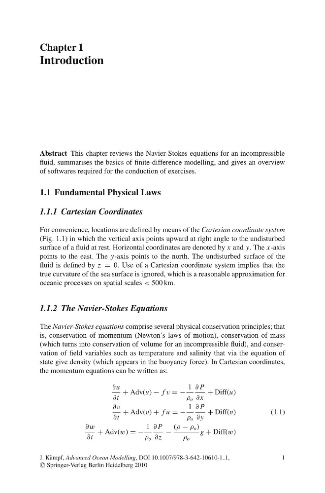
the momentum equations can be written as:
∂u
∂t
+ Adv(u) − f v = −
1
ρ o
∂ P
∂ x
+ Diff(u)
∂v
∂t
+ Adv(v) + f u = −
1
ρ o
∂ P
∂ y
+ Diff(v)
(1.1)
∂w
∂t
+ Adv(w) = −
1
ρ o
∂ P
∂z
−
(ρ − ρ o )
ρ o
g + Diff(w)
J. K¨ ampf, Advanced Ocean Modelling, DOI 10.1007/978-3-642-10610-1 1,
C
Springer-Verlag Berlin Heidelberg 2010
1
Introduction
Abstract This chapter reviews the Navier-Stokes equations for an incompressible
fluid, summarises the basics of finite-difference modelling, and gives an overview
of softwares required for the conduction of exercises.
1.1 Fundamental Physical Laws
1.1.1 Cartesian Coordinates
For convenience, locations are defined by means of the Cartesian coordinate system
(Fig. 1.1) in which the vertical axis points upward at right angle to the undisturbed
surface of a fluid at rest. Horizontal coordinates are denoted by x and y. The x-axis
points to the east. The y-axis points to the north. The undisturbed surface of the
fluid is defined by z = 0. Use of a Cartesian coordinate system implies that the
true curvature of the sea surface is ignored, which is a reasonable approximation for
oceanic processes on spatial scales < 500 km.
1.1.2 The Navier-Stokes Equations
The Navier-Stokes equations comprise several physical conservation principles; that
is, conservation of momentum (Newton’s laws of motion), conservation of mass
(which turns into conservation of volume for an incompressible fluid), and conservation of field variables such as temperature and salinity that via the equation of
state give density (which appears in the buoyancy force). In Cartesian coordinates,
the momentum equations can be written as:
∂u
∂t
+ Adv(u) − f v = −
1
ρ o
∂ P
∂ x
+ Diff(u)
∂v
∂t
+ Adv(v) + f u = −
1
ρ o
∂ P
∂ y
+ Diff(v)
(1.1)
∂w
∂t
+ Adv(w) = −
1
ρ o
∂ P
∂z
−
(ρ − ρ o )
ρ o
g + Diff(w)
J. K¨ ampf, Advanced Ocean Modelling, DOI 10.1007/978-3-642-10610-1 1,
C
Springer-Verlag Berlin Heidelberg 2010
1