

5.4 Exercise 21: Eddy Formation in a Strait
135
net. The General Bathymetric Chart of the Oceans (GEBCO) found at http://www.
gebco.net would be a useful data source. Instead of this, the author wishes to demonstrate the reader an alternative way to create an idealised bottom topography using
bathymetric charts as visual template. Section 5.4.4 details the method creating the
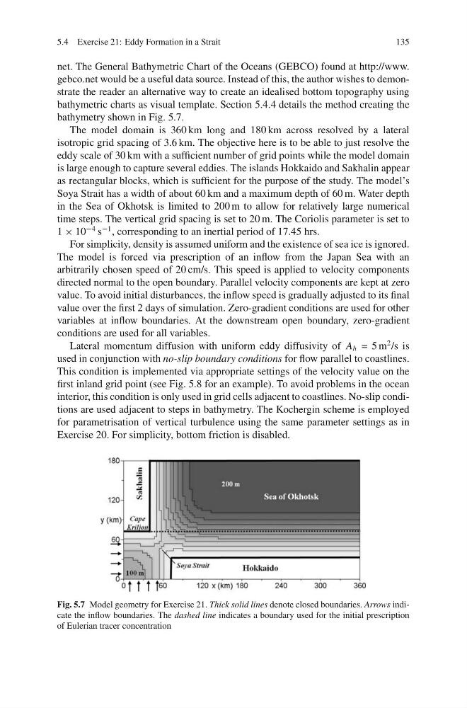
bathymetry shown in Fig. 5.7.
The model domain is 360 km long and 180 km across resolved by a lateral
isotropic grid spacing of 3.6 km. The objective here is to be able to just resolve the
eddy scale of 30 km with a sufficient number of grid points while the model domain
is large enough to capture several eddies. The islands Hokkaido and Sakhalin appear
as rectangular blocks, which is sufficient for the purpose of the study. The model’s
Soya Strait has a width of about 60 km and a maximum depth of 60 m. Water depth
in the Sea of Okhotsk is limited to 200 m to allow for relatively large numerical
time steps. The vertical grid spacing is set to 20 m. The Coriolis parameter is set to
1 × 10
−4 s
−1 , corresponding to an inertial period of 17.45 hrs.
For simplicity, density is assumed uniform and the existence of sea ice is ignored.
The model is forced via prescription of an inflow from the Japan Sea with an
arbitrarily chosen speed of 20 cm/s. This speed is applied to velocity components
directed normal to the open boundary. Parallel velocity components are kept at zero
value. To avoid initial disturbances, the inflow speed is gradually adjusted to its final
value over the first 2 days of simulation. Zero-gradient conditions are used for other
variables at inflow boundaries. At the downstream open boundary, zero-gradient
conditions are used for all variables.
Lateral momentum diffusion with uniform eddy diffusivity of A h = 5 m
2 /s is
used in conjunction with no-slip boundary conditions for flow parallel to coastlines.
This condition is implemented via appropriate settings of the velocity value on the
first inland grid point (see Fig. 5.8 for an example). To avoid problems in the ocean
interior, this condition is only used in grid cells adjacent to coastlines. No-slip conditions are used adjacent to steps in bathymetry. The Kochergin scheme is employed
for parametrisation of vertical turbulence using the same parameter settings as in
Exercise 20. For simplicity, bottom friction is disabled.
Fig. 5.7 Model geometry for Exercise 21. Thick solid lines denote closed boundaries. Arrows indicate the inflow boundaries. The dashed line indicates a boundary used for the initial prescription
of Eulerian tracer concentration
135
net. The General Bathymetric Chart of the Oceans (GEBCO) found at http://www.
gebco.net would be a useful data source. Instead of this, the author wishes to demonstrate the reader an alternative way to create an idealised bottom topography using
bathymetric charts as visual template. Section 5.4.4 details the method creating the
bathymetry shown in Fig. 5.7.
The model domain is 360 km long and 180 km across resolved by a lateral
isotropic grid spacing of 3.6 km. The objective here is to be able to just resolve the
eddy scale of 30 km with a sufficient number of grid points while the model domain
is large enough to capture several eddies. The islands Hokkaido and Sakhalin appear
as rectangular blocks, which is sufficient for the purpose of the study. The model’s
Soya Strait has a width of about 60 km and a maximum depth of 60 m. Water depth
in the Sea of Okhotsk is limited to 200 m to allow for relatively large numerical
time steps. The vertical grid spacing is set to 20 m. The Coriolis parameter is set to
1 × 10
−4 s
−1 , corresponding to an inertial period of 17.45 hrs.
For simplicity, density is assumed uniform and the existence of sea ice is ignored.
The model is forced via prescription of an inflow from the Japan Sea with an
arbitrarily chosen speed of 20 cm/s. This speed is applied to velocity components
directed normal to the open boundary. Parallel velocity components are kept at zero
value. To avoid initial disturbances, the inflow speed is gradually adjusted to its final
value over the first 2 days of simulation. Zero-gradient conditions are used for other
variables at inflow boundaries. At the downstream open boundary, zero-gradient
conditions are used for all variables.
Lateral momentum diffusion with uniform eddy diffusivity of A h = 5 m
2 /s is
used in conjunction with no-slip boundary conditions for flow parallel to coastlines.
This condition is implemented via appropriate settings of the velocity value on the
first inland grid point (see Fig. 5.8 for an example). To avoid problems in the ocean
interior, this condition is only used in grid cells adjacent to coastlines. No-slip conditions are used adjacent to steps in bathymetry. The Kochergin scheme is employed
for parametrisation of vertical turbulence using the same parameter settings as in
Exercise 20. For simplicity, bottom friction is disabled.
Fig. 5.7 Model geometry for Exercise 21. Thick solid lines denote closed boundaries. Arrows indicate the inflow boundaries. The dashed line indicates a boundary used for the initial prescription
of Eulerian tracer concentration