

136
5 3D Level Modelling
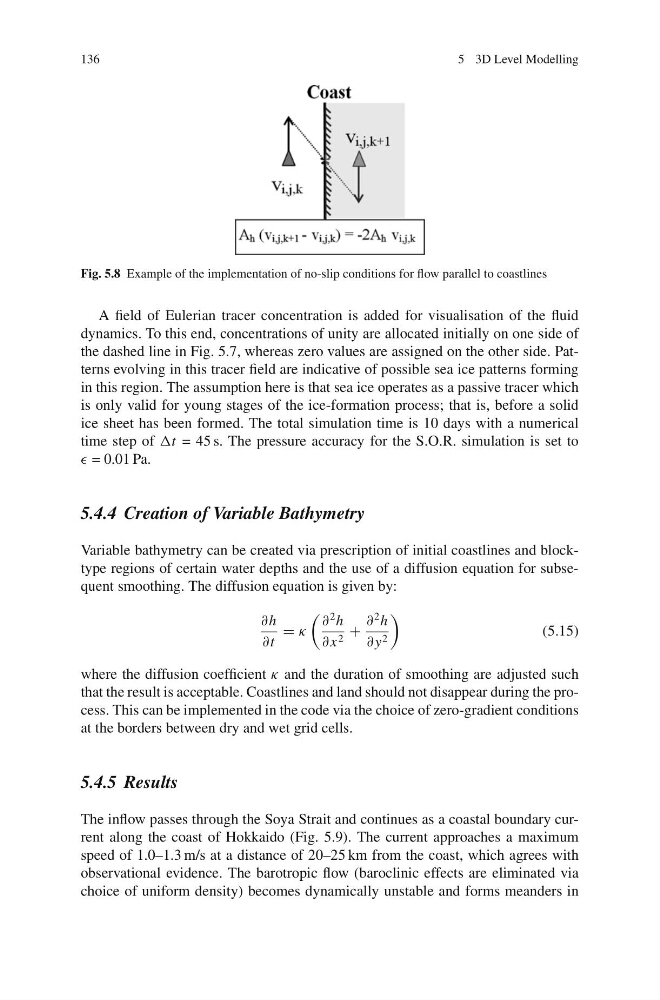
Fig. 5.8 Example of the implementation of no-slip conditions for flow parallel to coastlines
A field of Eulerian tracer concentration is added for visualisation of the fluid
dynamics. To this end, concentrations of unity are allocated initially on one side of
the dashed line in Fig. 5.7, whereas zero values are assigned on the other side. Patterns evolving in this tracer field are indicative of possible sea ice patterns forming
in this region. The assumption here is that sea ice operates as a passive tracer which
is only valid for young stages of the ice-formation process; that is, before a solid
ice sheet has been formed. The total simulation time is 10 days with a numerical
time step of Δt = 45 s. The pressure accuracy for the S.O.R. simulation is set to
= 0.01 Pa.
5.4.4 Creation of Variable Bathymetry
Variable bathymetry can be created via prescription of initial coastlines and blocktype regions of certain water depths and the use of a diffusion equation for subsequent smoothing. The diffusion equation is given by:
∂h
∂t
= κ
∂
2 h
∂ x 2 +
∂
2 h
∂ y 2
(5.15)
where the diffusion coefficient κ and the duration of smoothing are adjusted such
that the result is acceptable. Coastlines and land should not disappear during the process. This can be implemented in the code via the choice of zero-gradient conditions
at the borders between dry and wet grid cells.
5.4.5 Results
The inflow passes through the Soya Strait and continues as a coastal boundary current along the coast of Hokkaido (Fig. 5.9). The current approaches a maximum
speed of 1.0–1.3 m/s at a distance of 20–25 km from the coast, which agrees with
observational evidence. The barotropic flow (baroclinic effects are eliminated via
choice of uniform density) becomes dynamically unstable and forms meanders in
5 3D Level Modelling
Fig. 5.8 Example of the implementation of no-slip conditions for flow parallel to coastlines
A field of Eulerian tracer concentration is added for visualisation of the fluid
dynamics. To this end, concentrations of unity are allocated initially on one side of
the dashed line in Fig. 5.7, whereas zero values are assigned on the other side. Patterns evolving in this tracer field are indicative of possible sea ice patterns forming
in this region. The assumption here is that sea ice operates as a passive tracer which
is only valid for young stages of the ice-formation process; that is, before a solid
ice sheet has been formed. The total simulation time is 10 days with a numerical
time step of Δt = 45 s. The pressure accuracy for the S.O.R. simulation is set to
= 0.01 Pa.
5.4.4 Creation of Variable Bathymetry
Variable bathymetry can be created via prescription of initial coastlines and blocktype regions of certain water depths and the use of a diffusion equation for subsequent smoothing. The diffusion equation is given by:
∂h
∂t
= κ
∂
2 h
∂ x 2 +
∂
2 h
∂ y 2
(5.15)
where the diffusion coefficient κ and the duration of smoothing are adjusted such
that the result is acceptable. Coastlines and land should not disappear during the process. This can be implemented in the code via the choice of zero-gradient conditions
at the borders between dry and wet grid cells.
5.4.5 Results
The inflow passes through the Soya Strait and continues as a coastal boundary current along the coast of Hokkaido (Fig. 5.9). The current approaches a maximum
speed of 1.0–1.3 m/s at a distance of 20–25 km from the coast, which agrees with
observational evidence. The barotropic flow (baroclinic effects are eliminated via
choice of uniform density) becomes dynamically unstable and forms meanders in