

106
4 2.5D Vertical Slice Modelling
4.3 Exercise 17: Tidal-Mixing Fronts
4.3.1 Background
Tidal currents, if energetic enough, can trigger vertical mixing of the entire
water column. This tidal mixing only occurs in shallower regions of swift tidal flows,
whereas the density stratification in adjacent deeper portions of the sea and weaker
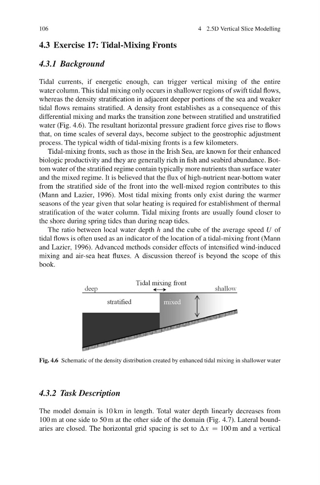
tidal flows remains stratified. A density front establishes as a consequence of this
differential mixing and marks the transition zone between stratified and unstratified
water (Fig. 4.6). The resultant horizontal pressure gradient force gives rise to flows
that, on time scales of several days, become subject to the geostrophic adjustment
process. The typical width of tidal-mixing fronts is a few kilometers.
Tidal-mixing fronts, such as those in the Irish Sea, are known for their enhanced
biologic productivity and they are generally rich in fish and seabird abundance. Bottom water of the stratified regime contain typically more nutrients than surface water
and the mixed regime. It is believed that the flux of high-nutrient near-bottom water
from the stratified side of the front into the well-mixed region contributes to this
(Mann and Lazier, 1996). Most tidal mixing fronts only exist during the warmer
seasons of the year given that solar heating is required for establishment of thermal
stratification of the water column. Tidal mixing fronts are usually found closer to
the shore during spring tides than during neap tides.
The ratio between local water depth h and the cube of the average speed U of
tidal flows is often used as an indicator of the location of a tidal-mixing front (Mann
and Lazier, 1996). Advanced methods consider effects of intensified wind-induced
mixing and air-sea heat fluxes. A discussion thereof is beyond the scope of this
book.
Fig. 4.6 Schematic of the density distribution created by enhanced tidal mixing in shallower water
4.3.2 Task Description
The model domain is 10 km in length. Total water depth linearly decreases from
100 m at one side to 50 m at the other side of the domain (Fig. 4.7). Lateral boundaries are closed. The horizontal grid spacing is set to Δx = 100 m and a vertical
4 2.5D Vertical Slice Modelling
4.3 Exercise 17: Tidal-Mixing Fronts
4.3.1 Background
Tidal currents, if energetic enough, can trigger vertical mixing of the entire
water column. This tidal mixing only occurs in shallower regions of swift tidal flows,
whereas the density stratification in adjacent deeper portions of the sea and weaker
tidal flows remains stratified. A density front establishes as a consequence of this
differential mixing and marks the transition zone between stratified and unstratified
water (Fig. 4.6). The resultant horizontal pressure gradient force gives rise to flows
that, on time scales of several days, become subject to the geostrophic adjustment
process. The typical width of tidal-mixing fronts is a few kilometers.
Tidal-mixing fronts, such as those in the Irish Sea, are known for their enhanced
biologic productivity and they are generally rich in fish and seabird abundance. Bottom water of the stratified regime contain typically more nutrients than surface water
and the mixed regime. It is believed that the flux of high-nutrient near-bottom water
from the stratified side of the front into the well-mixed region contributes to this
(Mann and Lazier, 1996). Most tidal mixing fronts only exist during the warmer
seasons of the year given that solar heating is required for establishment of thermal
stratification of the water column. Tidal mixing fronts are usually found closer to
the shore during spring tides than during neap tides.
The ratio between local water depth h and the cube of the average speed U of
tidal flows is often used as an indicator of the location of a tidal-mixing front (Mann
and Lazier, 1996). Advanced methods consider effects of intensified wind-induced
mixing and air-sea heat fluxes. A discussion thereof is beyond the scope of this
book.
Fig. 4.6 Schematic of the density distribution created by enhanced tidal mixing in shallower water
4.3.2 Task Description
The model domain is 10 km in length. Total water depth linearly decreases from
100 m at one side to 50 m at the other side of the domain (Fig. 4.7). Lateral boundaries are closed. The horizontal grid spacing is set to Δx = 100 m and a vertical